How much AMR obstacle avoidance latency is too much?

In AMR deployment, obstacle detection is only half the equation—response speed determines whether navigation stays safe, efficient, and production-ready. Understanding amr obstacle avoidance latency helps explain why two robots with similar sensors can perform very differently on the floor.

Latency is not a marketing detail. It directly affects stopping distance, false evasive actions, aisle congestion, and mission completion time. In dense industrial environments, even small timing delays can multiply into safety exposure and lost throughput.

This guide explains how much delay is too much, what metrics matter, and how to evaluate amr obstacle avoidance latency using engineering logic rather than vendor adjectives.

What does AMR obstacle avoidance latency actually include?

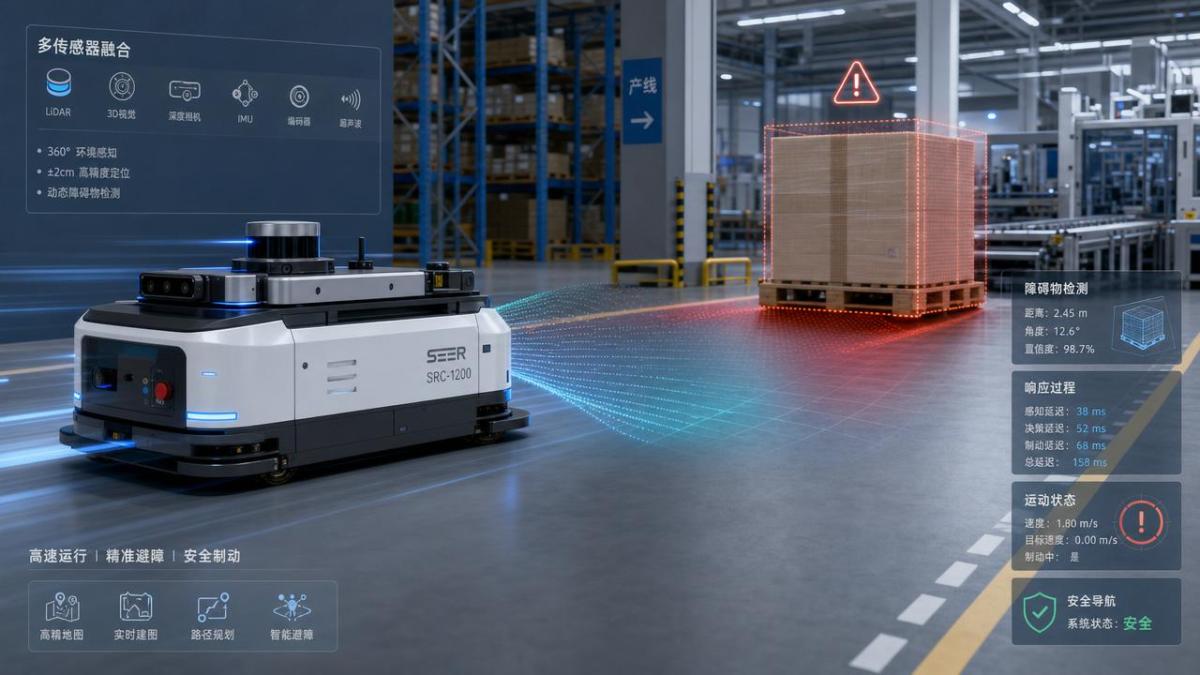
Many teams treat latency as one number. In reality, amr obstacle avoidance latency is a chain of delays across sensing, computing, decision-making, and motion execution.

A practical latency stack often includes:

• Sensor acquisition time from LiDAR, camera, radar, or depth modules
• Data filtering and object classification delay
• Path planning or local avoidance computation time
• Controller communication and safety interlock delay
• Brake or motor response after the command is issued

This means the published sensor refresh rate alone is not enough. A fast LiDAR with slow compute or weak braking can still produce poor real-world avoidance behavior.

TSV-style engineering review should separate detection latency, decision latency, and actuation latency. Only the combined end-to-end value describes usable amr obstacle avoidance latency.

How much AMR obstacle avoidance latency is too much?

There is no universal threshold. The acceptable value depends on speed, payload, floor condition, traffic density, and obstacle unpredictability.

Still, the engineering principle is simple: latency becomes too much when the robot cannot maintain a safe stopping or rerouting margin under worst-case operating conditions.

A useful formula is:

Total reaction distance = speed × total latency + braking distance

For example, an AMR moving at 1.8 m/s with 250 ms total latency travels 0.45 meters before braking even begins. That can already consume most of the clearance in narrow aisles.

If payload is heavy or the floor has low friction, braking distance grows further. In such cases, 250 ms may be tolerable in open areas but dangerous near intersections or work cells.

As a rough operating reference:

• Under 100 ms: strong for dynamic environments and faster AMRs
• 100–200 ms: often workable with controlled traffic and tuned motion limits
• 200–300 ms: requires careful validation and more conservative speeds
• Over 300 ms: frequently problematic in mixed traffic or tight industrial layouts

These are not certification limits. They are practical benchmarking bands for discussing amr obstacle avoidance latency in realistic operations.

Which operating scenarios make latency more critical?

Not every site has the same tolerance for delay. Some applications can absorb modest latency. Others cannot.

High-risk scenarios

• Mixed pedestrian and robot traffic
• Blind corners and cross-aisle intersections
• High-speed transport missions
• Heavy payload handling with longer stopping distance
• Reflective, dusty, or variable lighting environments

Lower-risk scenarios

• Low-speed line-side replenishment
• Wide aisles with predictable traffic patterns
• Restricted access zones with fixed workflows

The same amr obstacle avoidance latency value can therefore be acceptable in one site and unacceptable in another. Context matters more than brochure numbers.

This is especially true in comprehensive industrial settings, where AMRs may move between warehousing, assembly, kitting, inspection, and packaging areas in one shift.

How can you judge vendor claims beyond a single latency number?

A vendor may quote “response in 80 ms” without clarifying what is measured. That figure might describe only perception software, not total obstacle avoidance performance.

To evaluate amr obstacle avoidance latency properly, request test definitions and boundary conditions. Important questions include:

1. Is the number sensor-only or end-to-end?
2. What robot speed was used during the test?
3. What obstacle size, material, and approach angle were used?
4. Was the test static or dynamic?
5. Does the result include controller and brake delay?
6. What is the 95th percentile or worst-case latency?

Average values can hide dangerous spikes. A robot with 90 ms average latency but occasional 320 ms peaks may perform worse than a robot with stable 140 ms response.

Consistency is often more valuable than isolated best-case speed. For production deployment, jitter and tail latency deserve the same attention as nominal latency.

What technical factors most often increase AMR obstacle avoidance latency?

Slow response usually comes from system interaction, not one weak component. Several common causes appear repeatedly in field validation.

1. Sensor fusion overload

Combining LiDAR, cameras, and depth sensors improves coverage. It also increases processing demand. If compute resources are undersized, amr obstacle avoidance latency rises quickly.

2. Heavy AI inference pipelines

Complex object classification models can improve semantic understanding. Yet they may slow response if the platform lacks GPU efficiency or edge optimization.

3. Poor safety-controller integration

A fast detection stack is wasted if commands pass through slow middleware, weak network timing, or layered safety logic with unnecessary buffering.

4. Mechanical braking limits

Some robots decide quickly but stop slowly. Wheel traction, motor tuning, load distribution, and brake calibration all influence effective response.

5. Conservative software tuning

Excessive filtering may reduce false positives, but it can also delay action. Over-smoothed obstacle tracking can make the system appear stable while reducing real safety margin.

How should AMR obstacle avoidance latency be tested on site?

Factory acceptance data is useful, but site testing is essential. Real floors contain clutter, lighting variation, pallets, reflective wraps, and human movement patterns that lab tests rarely capture.

A practical validation approach should include:

• Static obstacle emergence tests at multiple speeds
• Dynamic crossing tests with controlled moving targets
• Loaded versus unloaded braking comparisons
• Corner-entry and intersection scenarios
• Repeatability measurement across many cycles

Record not only collision avoidance success. Also capture stop initiation time, deceleration profile, reroute smoothness, and recovery time after obstacle clearance.

This wider dataset shows whether amr obstacle avoidance latency hurts throughput even when collisions never occur. Excessively cautious robots can still damage productivity.

What are the most common mistakes when interpreting latency?

Several misconceptions distort AMR selection and deployment planning.

• Mistake 1: treating sensor frame rate as total response time
• Mistake 2: using average latency without worst-case distribution
• Mistake 3: ignoring payload and floor friction effects
• Mistake 4: assuming slower AMRs always solve latency risk
• Mistake 5: separating safety from throughput analysis

In reality, amr obstacle avoidance latency is both a safety metric and a productivity metric. Late response causes emergency stops. Overly defensive tuning causes hesitation and traffic waves.

The best system avoids both extremes: unsafe delay and unnecessary caution.

FAQ table: how to benchmark acceptable latency

The right question is not simply, “What is the latency?” The better question is, “What total amr obstacle avoidance latency remains under worst-case conditions, and how does it affect safe throughput?”

For any advanced automation program, that is the number worth validating. Use site-specific tests, demand end-to-end definitions, and compare consistency instead of headline claims alone.

At TSV, engineering truth starts with measurable parameters. When reviewing AMR fleets, quantify latency, stopping distance, and recovery behavior together. That approach turns obstacle avoidance from a brochure feature into a dependable operational benchmark.