Machine vision sub-pixel accuracy can fail on unstable lighting

Machine vision sub-pixel accuracy can collapse under unstable lighting, even when optics and algorithms appear nominal on paper. For engineers, operators, buyers, and decision-makers, this makes machine vision sub-pixel accuracy, machine vision lens distortion test, and lidar sunlight interference resistance critical evaluation points when validating real-world sensing performance.

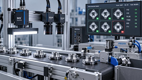
In industrial inspection, robotic guidance, UAV payload sensing, and edge AI measurement workflows, laboratory specifications often look better than production-floor results. A system rated for sub-pixel measurement may drift from repeatable detection at 0.1 pixel to unstable outputs several times worse once illumination fluctuates, reflective parts enter the field of view, or sunlight leaks into the sensing path.

For B2B teams working with precision manufacturing, automation, aerospace components, and smart sensing infrastructure, the core question is not whether a camera, lens, or LiDAR worked in a controlled demo. The real question is whether it remains stable across 3 shifts, changing ambient light, mixed materials, and variable operator handling. That is where engineering truth matters more than brochure language.

This article examines why sub-pixel performance degrades under unstable lighting, how a machine vision lens distortion test should be interpreted in procurement and validation, and why lidar sunlight interference resistance belongs in the same evaluation framework. The goal is to help information researchers, operators, buyers, and enterprise decision-makers build more reliable sensing selection criteria.

Why sub-pixel accuracy fails outside the lab

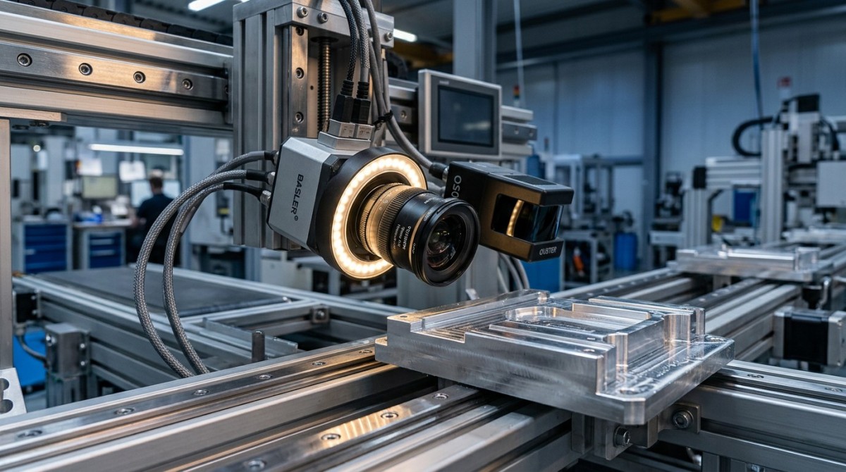
Sub-pixel accuracy is a mathematical refinement of edge or feature localization below one full pixel. In a stable setup, this can support measurement repeatability in the range of 0.05 to 0.25 pixel, depending on contrast, optics, calibration quality, and image processing. The problem is that the method assumes the image profile remains sufficiently consistent from frame to frame.

Unstable lighting breaks that assumption first by changing contrast gradients. If an edge that was previously sharp becomes partially washed out or shadowed, the calculated center of the transition shifts. Even a brightness variation of 10% to 20% across the region of interest can alter edge fitting results enough to move a dimensional reading beyond tolerance in high-precision applications.

Second, unstable lighting changes noise behavior. Short exposure times may increase sensor noise, while long exposure times may introduce blur from conveyor vibration or robotic motion. In systems measuring hole position, bead width, connector alignment, or solder geometry, that tradeoff can turn a nominal ±0.02 mm process window into repeated false rejects or false accepts.

Third, optical performance is often evaluated separately from illumination, even though they are tightly coupled. A lens that looks acceptable in a static chart test may respond very differently with specular metal, black rubber, carbon fiber weave, or transparent films. This is why machine vision sub-pixel accuracy should never be judged from resolution claims alone.

Three failure mechanisms seen in production lines

• Contrast drift: LED aging, voltage instability, ambient daylight, or dirty covers reduce edge definition over 2 to 12 weeks of operation.
• Geometry distortion under real setup conditions: focus shift, thermal expansion, and mounting stress modify image geometry after several hours of machine runtime.
• Algorithm sensitivity: threshold-based or profile-based tools may remain stable in one lot but become unreliable when surface finish varies by 5% to 15%.

What operators usually observe first

Operators rarely describe the problem as “sub-pixel collapse.” They report practical symptoms: more teach-ins per week, drifting measurements after lunch shift, vision alarms during bright afternoons, or inconsistent pass/fail decisions between line 1 and line 2. These symptoms are valuable because they point to environmental instability, not necessarily a bad camera.

For procurement teams, this distinction matters. Replacing the camera without checking illumination uniformity, lens distortion under installation load, and shielding against sunlight can increase cost while leaving the root cause unresolved.

How to evaluate machine vision lens distortion test results correctly

A machine vision lens distortion test is often treated as a one-time optical qualification. In reality, it should be part of a broader system validation process. Distortion affects how straight lines, spacing, and dimensions are mapped across the image field. In metrology or guidance tasks, even small residual distortion can bias sub-pixel calculations differently at the center and at the edge of the frame.

Many buyers focus on quoted distortion percentages such as below 0.1% or 0.05%. Those figures are useful, but they are incomplete unless the test conditions are defined. You need to know sensor size, working distance, aperture, target flatness, field coverage, and calibration method. A lens can perform well at one magnification ratio and degrade materially at another.

A practical evaluation should include at least 3 zones: center, mid-field, and edge. It should also compare distortion before and after installation, because mechanical stress from locking rings, adapters, or enclosure heat can slightly alter imaging geometry. In precision inspection, that small shift can be enough to push measurement uncertainty beyond acceptable limits.

For teams aligning TSV-style engineering benchmarking with supplier qualification, the key is to request distortion data in application context. Ask for repeatability under the intended standoff distance, illumination angle, and production speed rather than isolated optical marketing values.

Recommended lens distortion validation checklist

The table below shows a practical way to review machine vision lens distortion test data before approving a system for measurement, robotic positioning, or high-speed inspection.

The main conclusion is simple: a machine vision lens distortion test is only meaningful when tied to installation, thermal behavior, and usable field geometry. For buyers, this turns a generic lens comparison into a true risk-control exercise.

Common procurement mistake

A frequent error is selecting lenses by megapixel rating alone. A 12 MP or 20 MP lens may still underperform in sub-pixel applications if distortion compensation is weak at the actual field edge or if aperture choice reduces contrast stability. Resolution supports measurement, but it does not guarantee measurement integrity.

Why lidar sunlight interference resistance belongs in the same decision framework

Machine vision and LiDAR are often sourced by different teams, but both are vulnerable to unstable optical environments. For LiDAR, bright sunlight introduces optical noise, false returns, reduced contrast against low-reflectivity targets, and range instability at certain angles. In outdoor logistics, UAV perception, and yard automation, this can be just as disruptive as unstable lighting in a camera-based metrology station.

Lidar sunlight interference resistance should be assessed not only by maximum range, but by stable detection under illumination stress. A unit may claim 100 m or 200 m nominal range, yet experience substantial degradation under midday sun, high albedo surfaces, or dusty air. For many industrial users, the more useful metric is not peak distance but repeatable detection confidence at the operating threshold.

This matters especially in mixed sensing architectures. A mobile robot may use machine vision for feature recognition and LiDAR for navigation. If the vision system is disturbed by internal lighting changes while the LiDAR is disturbed by sunlight ingress at dock doors, the combined system can fail in ways not visible during commissioning week.

A TSV-style benchmarking mindset treats both technologies as parts of one sensing reliability chain. The evaluation focus should be anti-interference behavior, repeatability, and environmental tolerance, not just ideal-condition performance.

Comparison of optical interference risks

The following table helps cross-functional teams compare how unstable light affects machine vision and LiDAR in procurement and deployment planning.

The practical takeaway is that sunlight resistance, contrast stability, and contamination control should be specified early. Otherwise, system integration teams may spend 2 to 6 months fixing environmental issues that should have been screened during vendor qualification.

When this matters most

• Dock doors, skylit workshops, and outdoor transfer points where ambient illumination can shift within 15 to 30 minutes.
• UAV mapping or infrastructure inspection where sun angle changes data density and feature consistency through a single mission.
• AMR, AGV, and robotic cells combining cameras, LiDAR, and edge AI where one unstable sensor degrades the full decision chain.

Selection and validation criteria for engineers, operators, buyers, and decision-makers

Different stakeholders look at sensing performance through different lenses. Engineers prioritize calibration repeatability and algorithm robustness. Operators care about ease of maintenance and alarm stability. Buyers need comparable technical criteria across suppliers. Decision-makers want lower trial-and-error cost and shorter qualification cycles. A workable framework must satisfy all four groups at the same time.

The first rule is to test in conditions that approximate production. That means evaluating systems across at least 3 lighting states: nominal, low-light, and high-glare or sun-exposed. If the application is outdoor or near open doors, include morning and midday conditions. If the line runs 16 to 24 hours, add warm-state verification after thermal stabilization.

The second rule is to convert optical claims into operational criteria. Instead of asking whether a camera supports sub-pixel accuracy, ask what repeatability it maintains after 8 hours, after lens cleaning intervals, and under ±10% illuminance variation. Instead of asking whether LiDAR is sunlight resistant, ask how point cloud usefulness changes under direct sun at working angles relevant to your layout.

The third rule is to document acceptance thresholds before pilot deployment. This avoids subjective arguments later and helps procurement compare suppliers on measurable engineering performance rather than sales framing.

Core selection criteria by stakeholder

• Engineers: measurement repeatability, calibration drift, distortion compensation quality, and interference tolerance across 3 to 5 environmental states.
• Operators: cleaning frequency, teach-in stability, false alarm rate per shift, and time needed to recover after lighting or fixture changes.
• Buyers: defined test protocol, spare lead time, support response window, and evidence of validation under similar materials and speeds.
• Decision-makers: impact on scrap risk, commissioning time, line uptime, and supplier transparency on edge-case limitations.

A practical acceptance model

Many teams benefit from a 4-part acceptance model: optical baseline, environmental stress test, process integration trial, and maintenance stability review. This can be completed in 2 to 4 weeks for a focused pilot. The benefit is faster elimination of hidden risk before full rollout.

For example, if a measurement station targets ±0.03 mm repeatability, the validation should confirm whether that remains true after illumination fluctuation, contamination buildup, and 3 consecutive shift cycles. If not, the issue is not only optical quality but system resilience.

Implementation steps, common mistakes, and maintenance discipline

Reliable sensing performance is built through disciplined implementation. Even a strong component set can underperform if lighting geometry, shielding, mounting rigidity, and maintenance intervals are weak. In practice, the difference between a stable sub-pixel inspection cell and a troublesome one is often found in setup detail rather than in headline hardware specifications.

A useful deployment path begins with application mapping. Define object material, motion speed, target tolerance, environmental light sources, contamination sources, and allowable cycle time. Then match camera, lens, light, filters, and LiDAR only after those constraints are documented. This sequence reduces redesign loops and keeps qualification grounded in real operating physics.

Maintenance discipline is equally important. Illumination output may decline gradually over 1,000 to 10,000 operating hours depending on the source and environment. Transparent covers accumulate film. Lens mounts loosen with vibration. Calibration targets age or warp. Without periodic checks, systems drift slowly until operators notice instability long after process capability has already degraded.

For enterprises managing multiple plants or suppliers, a standardized verification routine creates major value. It shortens troubleshooting time, makes vendor comparison more objective, and turns sensing procurement into a controlled engineering process instead of a sequence of reactive fixes.

Recommended implementation flow

1. Define the measurement or detection target, including tolerance, speed, material, and expected environmental variation.
2. Run a baseline machine vision lens distortion test and illumination uniformity review at nominal setup.
3. Stress test under at least 3 lighting scenarios, including glare or sunlight exposure where relevant.
4. Validate lidar sunlight interference resistance if navigation, ranging, or outdoor sensing is part of the workflow.
5. Set maintenance checkpoints every 2 to 6 weeks based on contamination level, thermal load, and uptime.

Common mistakes to avoid

• Approving a vision system from static demo images without shift-based repeatability data.
• Treating lens distortion values as universal, even though performance changes with working distance and mounting conditions.
• Ignoring skylights, dock doors, and reflective machine surfaces during project planning.
• Assuming algorithm tuning can permanently fix hardware or environmental instability.
• Skipping maintenance logs, then losing traceability when drift appears after 6 to 8 weeks.

FAQ for sourcing and deployment teams

How should buyers compare machine vision sub-pixel accuracy across suppliers?

Compare repeatability under the same target, distance, exposure strategy, and lighting instability range. A valid comparison should include at least 30 to 50 repeated measurements per condition, not one ideal screenshot. Ask for raw variation and failure cases, not only best-case averages.

What is the minimum useful machine vision lens distortion test scope?

At minimum, test center and edge behavior, before and after installation, and after warm-up. If the task is dimensional metrology or robotic positioning, include calibration residuals and repeatability at nominal distance and at ±5% distance change.

When should lidar sunlight interference resistance be a priority?

It should be prioritized in outdoor applications, semi-open industrial areas, and any indoor route where sunlight enters directly. It also matters for AMRs, AGVs, UAVs, and perimeter monitoring systems where false returns or missed detections can affect safety or navigation quality.

Machine vision sub-pixel accuracy is valuable only when it survives real operating conditions. That is why machine vision lens distortion test data, lighting stability analysis, and lidar sunlight interference resistance should be reviewed as one integrated reliability problem rather than separate specification lines. For engineers, operators, buyers, and executives, this approach reduces hidden validation risk, shortens supplier screening cycles, and improves confidence in sensing deployment.

At TechStat Vanguard, the priority is practical engineering truth: measurable tolerances, testable interference limits, and decision frameworks that hold up beyond the demo environment. If you are qualifying sensing components, benchmarking suppliers, or building a more resilient machine vision and LiDAR evaluation process, now is the time to align procurement with real-world validation. Contact us to discuss your application, request a tailored evaluation framework, or learn more about data-driven hard-tech benchmarking solutions.