How Can You Fairly Compare MTBF Across Industrial Servo Motors?

A fair industrial servo motor MTBF comparison requires a common operating profile, a common definition of failure, and reliability evidence with comparable statistical confidence. A larger published figure cannot establish superiority when one motor was evaluated under light continuous rotation and another experienced repeated acceleration, high holding torque, or contamination.

Start by identifying what each number represents: observed operating history, a reliability demonstration, or a prediction assembled from component models. Then compare the conditions and uncertainty behind it. Where those foundations differ, the defensible outcome is an evidence gap rather than a ranking.

Define the failure boundary before comparing numbers

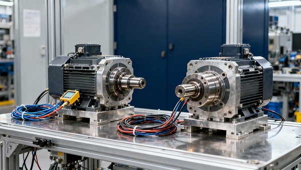
A servo motor includes several potential failure sources: bearings, winding insulation, feedback electronics, connectors, shaft seals, and an optional holding brake. A quoted MTBF might cover the motor assembly, the encoder alone, or a complete axis containing the drive and cables. Those figures describe different populations of failures.

The comparison boundary should specify the exact motor configuration and included components. A brake-equipped version cannot inherit the reliability claim of an otherwise similar motor without accounting for the brake and its operating conditions. Likewise, a feedback-device change can alter the evidence supporting the assembly even when torque and dimensions remain unchanged.

Failure also needs a functional definition. Complete loss of rotation is straightforward, but intermittent encoder errors, excessive bearing vibration, insulation deterioration, and inability to maintain positioning accuracy require explicit acceptance limits. Otherwise, one dataset records degradation as failure while another continues accumulating operating hours.

Distinguish a confirmed motor defect from an axis stoppage. A following-error trip might originate in mechanical binding, drive tuning, feedback interference, or a motor fault. Counting every trip against the motor inflates its apparent failure rate; excluding every resettable event hides intermittent faults. Record the event first, then classify its cause using agreed diagnostic evidence.

Match the mission profile, including the time spent holding position

“Operating at rated load” is insufficient detail for a servo application. The sequence of torque, speed, acceleration, dwell, and reversal determines the stresses experienced by the assembly. Two cycles with equal average torque can have different peak currents, bearing loads, and winding temperatures.

Include energized standstill in the profile. A motor holding a vertical load can generate substantial winding heat while accumulating no shaft revolutions. Conversely, bearing wear during sustained rotation follows a different exposure pattern. “Running hours” must therefore state whether the clock includes holding, powered idle, and unpowered downtime.

RMS torque helps characterize heating over a cycle, but it does not describe every reliability stress. Peak torque and its duration matter separately, as do speed-dependent losses and thermal cycling. A repeated short overload followed by cooling should not be treated as equivalent to continuous torque merely because a cycle average matches.

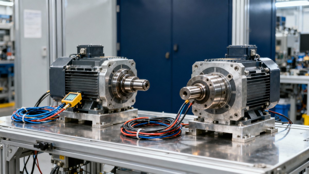
Mounting deserves particular attention. Heat conducted into a machine frame changes motor temperature, while belt tension and pulley overhang change bearing loading. A laboratory installation with a rigid, heat-dissipating flange and negligible shaft load provides limited evidence for a compact enclosed axis driving a tensioned belt.

Use the intended application cycle as the shared reference. Compare motors sized to perform that cycle within their specified limits, and record each motor’s utilization. Equal absolute torque represents different relative loading when continuous ratings differ; equal percentages of rated torque represent different delivered work. The comparison must identify which question it answers.

Separate observed reliability from modeled predictions

Field observations, controlled tests, and component-based predictions each answer different questions. Field data capture installation diversity and actual service events, but often contain incomplete operating records. Controlled testing makes conditions clearer, although the tested environment may cover only part of the intended application.

A modeled MTBF combines assumed component failure rates with a system model. Its usefulness depends on whether those rates, temperature assumptions, and interconnections represent the actual motor. It provides no direct proof that the complete assembly survived the stated duration.

A component model that assumes constant random failure rates also needs separate treatment of wear mechanisms. Bearing fatigue, lubricant deterioration, seal wear, and brake friction wear do not become adequately characterized simply by adding electronic component failure rates.

Keep predicted and observed figures in separate comparison columns. For a prediction, request the model basis, included parts, operating assumptions, and treatment of mechanical wear. For observed results, request the population, accumulated exposure, failure count, configuration history, and event-classification rules. Combining these evidence types into a single numerical ranking conceals their different meanings.

Read accumulated hours together with failures and confidence

Under a constant failure-rate model, a common MTBF estimate is total relevant operating exposure divided by the number of qualifying failures. Exposure is accumulated across the observed units; it is not necessarily the elapsed duration of the test. The estimate is meaningful only when the population and counting rules support that model.

MTBF estimate = total accumulated operating hours / qualifying failures

The failure count controls how much information supports that estimate. A result based on very few events carries substantial uncertainty, even when accumulated hours look impressive. Compare confidence intervals or confidence bounds, with the same confidence level and calculation method, alongside the point estimates.

Zero observed failures do not establish infinite MTBF. Under a constant-rate exponential model with independent exposure and complete failure detection, a one-sided lower confidence bound can be expressed as:

MTBF lower bound = total accumulated operating hours / [−ln(α)], where the confidence level is 1 − α.

This is a model-dependent bound, not an observed average interval between failures. Many units tested briefly can accumulate considerable exposure while revealing little about late-life bearing or insulation degradation. Preserve both total unit-hours and the distribution of individual operating ages.

Units that remain functioning at the end of observation contribute right-censored exposure. Excluding them wastes evidence. Units removed because of abnormal noise or intermittent faults need different treatment: labeling those removals as ordinary censoring can bias the result upward because removal was related to deterioration.

Repeated failures on the same repaired motor also require care. Replacing an encoder leaves the bearings and winding at their existing ages. Treating that repair as a completely new motor erases relevant history. State whether the analysis measures time to first failure, recurrent assembly failures, or failures after full replacement.

Do not use MTBF as a substitute for wear life

MTBF is commonly associated with repairable equipment, while mean time to failure describes a nonrepairable item’s time to failure. Published servo specifications sometimes use the terms loosely. Establish what was actually measured before applying either number to service-life planning.

A constant-rate model describes random failures over a specified operating region. Wear-out introduces an age-dependent failure rate. If failures cluster at later ages, a single MTBF obscures when the risk increases and cannot reliably define a replacement interval.

Bearing life ratings provide another distinct metric. A rating expressed at a specified survival percentage describes fatigue behavior under stated load assumptions. It does not automatically include lubricant breakdown, contamination, installation damage, encoder faults, or winding failure. Comparing that rating directly with assembly MTBF mixes different endpoints.

For wear-dominated evidence, compare survival at the required mission duration or a consistently defined life percentile. A Weibull analysis can describe changing failure behavior when the data support it, but fitted parameters need uncertainty estimates. Sparse observations do not justify a precise lifetime curve.

If the practical question is whether a motor will complete a scheduled service interval, request evidence at that interval. Converting MTBF into mission reliability through R(t) = exp(−t/MTBF) is valid only under the constant-rate exponential assumption. Applying it through an uncharacterized wear-out region produces misleading confidence.

Normalization needs a physical basis

Different test conditions sometimes permit adjustment, but no universal correction factor makes every servo MTBF comparable. Raising temperature affects winding insulation, lubricant, magnets, and electronics through different mechanisms. A temperature model validated for one mechanism does not automatically describe the complete assembly.

Accelerated testing should identify the failure mechanism being accelerated, demonstrate that it remains representative, and disclose the relationship used to translate exposure. Excessive temperature or load can introduce a failure mode absent from normal service, invalidating the extrapolation.

Bearing fatigue calculations can account for specified loads and speeds within their assumptions. They do not automatically normalize seal leakage or electrical feedback faults. Similarly, an electronics reliability prediction adjusted for temperature cannot correct for pulley misalignment.

Where validated adjustments are unavailable, group results by comparable conditions and leave unmatched claims unranked. A common controlled test resolves the gap more credibly than an undocumented correction. Record thermal histories and failure modes during that test so equal commanded cycles can be interpreted correctly.

Turn the evidence into a defensible comparison

Build the comparison record around the exact motor variant, application profile, evidence source, exposure, failures, and uncertainty. Keep differences visible instead of compressing everything into a score. A claim with missing failure definitions or unidentified test conditions remains unsuitable for direct ranking, regardless of its numerical size.

When two point estimates differ but their uncertainty ranges overlap substantially, the available evidence may not support a clear ordering. Overlap alone is not a formal significance test; a stronger claim requires an appropriate statistical comparison and compatible datasets. Report the unresolved difference instead of presenting the larger estimate as a proven advantage.

A useful acceptance requirement specifies the operating cycle, failure criteria, required mission duration, and statistical confidence before testing begins. It also defines how configuration changes, repairs, and early removals enter the record. That agreement makes the eventual result interpretable.

The final conclusion can be specific: stronger evidence under the matched application profile, demonstrated survival through the required interval, or insufficient comparable data. Each is more useful than an unsupported declaration that the motor with the highest advertised MTBF is the most reliable.