Edge AI inference latency in industrial vision tasks

In industrial vision systems, edge ai inference latency industrial is not just a speed metric—it directly affects detection accuracy, line stability, and ROI. For engineers, operators, buyers, and decision-makers evaluating vision based quality inspection software, this guide explains how latency interacts with hardware, models, and real-world deployment constraints to shape measurable production performance.

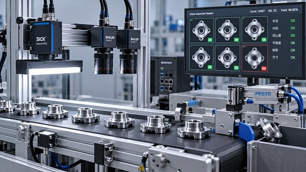
Across automated inspection, robotic guidance, packaging verification, and high-mix manufacturing, latency determines whether an image becomes a useful decision in time. A system that reports a defect 20 milliseconds too late may still be technically accurate, but operationally useless when a conveyor runs at 0.8–2.0 m/s or when a pick-and-place robot cycles in less than 500 ms.

For TSV’s audience, the key question is not whether an edge AI device is “fast.” The question is how much end-to-end delay exists between image capture, preprocessing, model inference, decision output, and actuator response—and whether that delay remains stable over 8-hour, 16-hour, or 24/7 production conditions.

This article focuses on practical engineering truths: what latency really includes, what thresholds matter by application, how to evaluate trade-offs between model complexity and line speed, and what procurement teams should verify before investing in industrial vision infrastructure.

What edge AI inference latency means in industrial vision

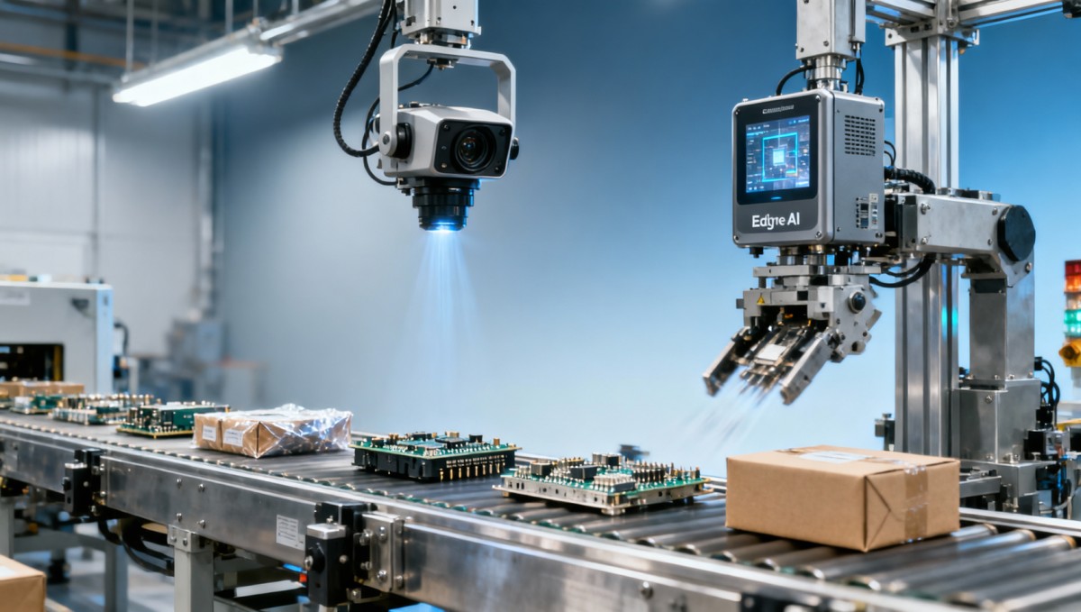
In factory environments, inference latency is often misunderstood as the model runtime alone. In reality, industrial vision latency is usually the sum of at least 5 stages: image acquisition, image transfer, preprocessing, neural network inference, and output communication to a PLC, robot controller, or edge gateway. In many deployments, the neural network itself accounts for only 30%–60% of total delay.

This distinction matters because a quoted “8 ms inference” from a chip vendor may translate into 22–45 ms end-to-end action time once camera trigger timing, memory movement, protocol overhead, and rejection gate actuation are included. On a line inspecting 120 parts per minute, that gap can determine whether the reject mechanism fires on the correct item or the next one.

In industrial settings, latency must also be evaluated together with jitter. A system averaging 18 ms but fluctuating between 12 ms and 35 ms may be harder to validate than a system fixed at 24 ms. Operators and controls engineers generally prefer predictable timing because deterministic behavior simplifies synchronization with encoders, strobes, conveyor tracking, and robot motion windows.

For procurement teams, this means performance comparisons should be based on consistent test conditions: input resolution, batch size, model type, ambient temperature, duty cycle, and interface protocol. A benchmark without those constraints does not support supplier qualification or line integration decisions.

Latency components engineers should separate

A clear breakdown improves both system design and vendor evaluation. Instead of asking for one headline number, teams should request time segmentation by function. This is especially important when comparing GPU-based edge boxes, FPGA systems, embedded NPUs, and industrial IPC platforms.

• Sensor exposure and trigger delay: commonly 1–10 ms depending on lighting and shutter strategy.
• Image transfer and buffering: often 2–15 ms depending on GigE Vision, USB3, MIPI, or CoaXPress architecture.
• Preprocessing time: typically 1–8 ms for resize, normalization, ROI extraction, or color conversion.
• Model inference time: often 5–40 ms at the edge, depending on network size and precision mode.
• Control output and actuation: usually 3–20 ms when PLC logic and mechanical response are included.

When these stages are measured independently, bottlenecks become visible. In some applications, reducing model size by 30% yields less benefit than replacing an overloaded camera interface or optimizing PLC polling intervals.

Why latency directly affects yield, uptime, and ROI

Industrial vision systems do not operate in isolation. They sit inside tightly timed production sequences where milliseconds accumulate into missed detections, false rejects, robot hesitation, or throughput loss. In surface inspection, cap presence verification, weld seam checking, or PCB defect screening, slow or unstable edge AI inference latency industrial can erode the business case even when model accuracy appears strong in offline testing.

Consider a conveyor application running at 1.2 m/s with a decision-to-actuation window of 50 mm. That leaves roughly 41.7 ms for the complete cycle from image capture to reject command. If actual system latency reaches 55 ms under peak load, the result may be mistimed rejection, manual rework, and traceability exceptions. Even a 2% increase in false rejects can become expensive on lines processing 20,000–50,000 units per shift.

For robotic guidance, latency changes coordinate relevance. A pose estimate produced 30 ms late may still be mathematically correct for the earlier frame, but physically wrong for a moving part. This is why many high-speed guidance applications target end-to-end timing under 25 ms, while slower assembly verification may tolerate 80–150 ms if decisions are not motion-critical.

From a financial perspective, buyers should link latency to measurable plant outcomes: scrap rate, first-pass yield, operator intervention frequency, and cycle time. A system that costs 15% more but avoids one extra stop per week or preserves 3% line throughput can produce a better payback over 12–24 months than a lower-cost but slower platform.

Typical latency tolerance by use case

Not every industrial vision task needs the same response time. The table below provides practical ranges that engineering and procurement teams can use during requirement definition.

These ranges are not universal specifications, but they provide a useful baseline. Final acceptance thresholds should be defined around line speed, object spacing, mechanical actuation delay, and the cost of a late or incorrect decision.

A common ROI mistake

A frequent procurement error is comparing systems on model accuracy only, such as 98.7% versus 99.1%, without checking whether both results were achieved at the same latency and image resolution. In production, a slightly lower accuracy model running at 18 ms can outperform a more complex model running at 60 ms if it enables stable line speed and lower intervention rates.

The engineering variables that drive latency at the edge

Edge AI inference latency industrial is shaped by a chain of interacting variables rather than one isolated hardware number. Camera resolution, exposure strategy, model architecture, accelerator type, thermal behavior, and communication stack all contribute. As a result, the same neural network can perform very differently across two edge devices even when vendor datasheets list similar TOPS or GPU memory figures.

Resolution is one of the biggest levers. Moving from 640×480 to 1920×1080 increases pixel count by more than 6 times, often multiplying preprocessing load and memory transfer time. If the inspection target occupies only 15% of the frame, a well-designed ROI pipeline can reduce overall latency more effectively than replacing the compute module.

Model choice also matters. A compact classifier or segmentation network optimized for INT8 inference may deliver 8–20 ms performance, while a larger transformer-based or multi-head detection model may require 30–80 ms on the same edge platform. The engineering challenge is to find the lowest-complexity model that still meets defect sensitivity, false-positive tolerance, and validation requirements.

Thermals are often underestimated. In enclosed factory cabinets operating at 35°C–45°C ambient temperature, some processors reduce frequency after sustained load, causing latency drift over a 2-hour to 6-hour period. This is why benchmark testing should include thermal soak and continuous-duty conditions, not only short laboratory bursts.

Key design factors and their practical effect

The following comparison helps teams connect engineering choices to deployment outcomes instead of relying on generic speed claims.

The critical conclusion is that latency optimization should start with system architecture, not only chipset selection. Many industrial projects overspend on compute because they do not first reduce unnecessary image and communication load.

A practical optimization sequence

1. Define the maximum allowed end-to-end latency from the production process backward.
2. Reduce image payload through optics, lighting, ROI, or trigger control.
3. Select the smallest model that meets validation thresholds.
4. Test under continuous duty for at least one full shift, preferably 8–12 hours.
5. Measure jitter, not only average latency.

This sequence usually produces a more reliable deployment than choosing the highest advertised compute density first and trying to correct integration issues later.

How buyers and decision-makers should evaluate edge vision platforms

For buyers, the challenge is turning technical complexity into a repeatable supplier evaluation process. A good procurement framework should verify not just whether the platform can run a demo, but whether it can sustain the required latency across the target application mix, maintenance cycle, and industrial environment. This is especially important in multi-line plants where one platform may need to support 3–10 different inspection recipes.

The first procurement principle is to request application-specific benchmarks. A supplier should test the actual image resolution, frame rate, model class, and response interface you intend to use. A generic benchmark at 224×224 or 640×640 is often insufficient for industrial inspection where cameras may run 2 MP, 5 MP, or higher and the decision path includes PLC signaling.

The second principle is to compare total cost of deployment, not only device cost. A lower-cost edge unit may require external cooling, custom integration, more frequent retraining, or additional engineering time to maintain line timing. In contrast, a better-matched system may reduce qualification time by 2–4 weeks and lower troubleshooting effort during ramp-up.

The third principle is serviceability. Operators and maintenance teams need diagnostics that show frame timing, dropped frames, inference queue depth, and communication delay. Without those visibility tools, even a technically capable system becomes hard to troubleshoot when latency shifts after model updates or production changes.

Procurement checklist for industrial edge AI vision

The table below converts engineering concerns into practical qualification criteria for sourcing teams, plant managers, and CTO-level reviewers.

A disciplined checklist helps separate marketing claims from deployable capability. This aligns with TSV’s broader view that parameters, tolerances, and sustained operating thresholds are more useful than generic superlatives during supplier selection.

Questions that should appear in every RFQ

• What is the measured trigger-to-output latency at the intended image size and model version?
• What is the 95th percentile and worst-case latency over extended runtime?
• What cooling or enclosure conditions are required to maintain that performance?
• How long does recipe changeover or model deployment typically take in production?
• What diagnostic data is available to operators and maintenance personnel?

These questions create a stronger technical-commercial basis for approval decisions, especially when CAPEX justification depends on reduced scrap, lower labor intervention, or faster supplier qualification.

Deployment strategy, risk control, and common mistakes

Successful deployment of low-latency industrial vision depends on disciplined staging. A practical implementation usually moves through 4 phases: requirement definition, controlled pilot, line integration, and sustained monitoring. Skipping any of these steps increases the chance that acceptable laboratory performance turns into unstable plant behavior after production launch.

During the pilot phase, teams should validate not only average inference time but also timing consistency under realistic workloads. This includes variable part appearance, lighting drift, operator interaction, and upstream speed changes. A pilot of 1–2 hours is rarely enough for high-confidence acceptance; many manufacturers benefit from a longer 1-shift or 3-shift validation before scaling.

A common mistake is overfitting the model to a clean dataset while ignoring production noise. Another is treating the edge device as a standalone AI component instead of part of a machine control system. In practice, camera trigger configuration, strobe timing, encoder mapping, buffer handling, and PLC scan time can each add enough delay to break a tightly timed process.

Risk control should therefore combine software and controls engineering. Acceptance criteria should include maximum latency, jitter threshold, missed-frame tolerance, and recovery behavior after network interruptions or recipe switches. For high-value applications, teams may also define fallback logic if inference exceeds a specified threshold such as 40 ms or 60 ms for more than a fixed number of cycles.

Frequent deployment mistakes

• Using average latency only and ignoring worst-case timing during peaks or thermal load.
• Selecting high-resolution cameras before confirming whether the defect actually requires that pixel density.
• Benchmarking with test images offline rather than full trigger-to-output measurements on the target line.
• Failing to coordinate AI timing with PLC scan cycles, reject mechanisms, and robot motion windows.
• Neglecting maintenance diagnostics, making post-deployment troubleshooting slow and expensive.

FAQ: Practical questions from engineers and buyers

How low should latency be for industrial vision? The answer depends on process timing. High-speed reject systems may require 10–30 ms end-to-end, while station-based inspection may tolerate 80–200 ms. The key is matching latency to the available decision window, not chasing the lowest possible number.

Is cloud inference acceptable for factory inspection? For non-critical analytics, sometimes yes. For motion-coupled inspection or real-time actuation, local edge inference is usually safer because network round-trip variability can add tens of milliseconds and increase timing uncertainty.

Should we prioritize a bigger model or lower latency? In most production lines, a balanced model with stable timing is preferable. A 99% accurate model that responds too slowly can create more cost than a 98% accurate model that holds timing consistently over 8–24 hour operation.

What is a reasonable validation duration before purchase approval? For many industrial scenarios, at least one full shift is a practical minimum. More demanding environments may require multiple shifts, product variants, and ambient temperature variation to ensure confidence.

Edge AI inference latency in industrial vision is ultimately a systems engineering issue, not just a processor specification. The most effective teams define timing limits from the process backward, validate end-to-end performance under real operating conditions, and procure platforms based on measurable stability rather than marketing language.

For information researchers, operators, sourcing teams, and enterprise decision-makers, the most reliable path is to compare latency, jitter, thermal behavior, integration fit, and serviceability as one package. That approach shortens trial-and-error cycles and improves the odds of achieving measurable gains in yield, uptime, and payback period.

If you are evaluating vision based quality inspection software, edge compute hardware, or supplier capability for industrial AI deployment, now is the right time to turn broad claims into parameter-based decisions. Contact us to discuss your application, request a tailored evaluation framework, or explore a more precise benchmarking approach for your production environment.