Edge AI latency in industry depends on more than the model

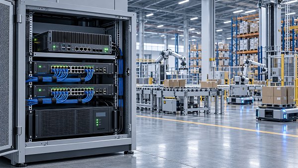
In industrial edge deployments, edge ai inference latency industrial is shaped not only by model size, but by the full data path—from sensor capture and agv traffic control algorithm to mqtt broker payload size limit, opc ua server response time, and 5g industrial router throughput test. For engineers, buyers, and decision-makers, understanding these bottlenecks is essential to selecting systems that deliver deterministic performance instead of marketing promises.

Why industrial edge AI latency is a system problem, not a model problem

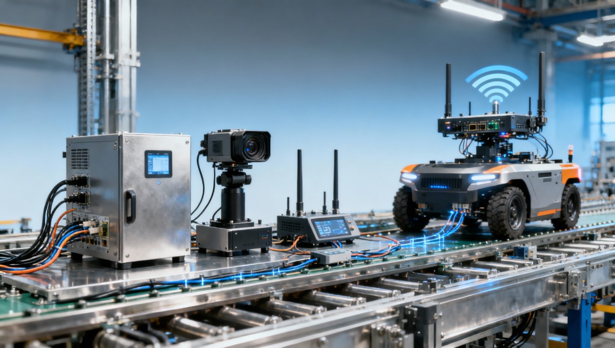
Many industrial teams start latency analysis at the neural network and stop there. That is rarely enough. In a real deployment, the end-to-end response path includes sensor exposure time, transport buffering, protocol conversion, message queue behavior, preprocessing, inference, postprocessing, and actuator or HMI feedback. A 15 ms model can still produce a 120 ms operational delay if the rest of the stack is not engineered for deterministic timing.

This matters across robotics, machine vision, AGV/AMR fleets, UAV ground systems, and industrial IoT gateways. In these environments, a latency difference of 20–50 ms may decide whether a robot keeps cycle time, whether a sorter misses an item, or whether an autonomous vehicle reacts before the next control window. For procurement teams, this means headline TOPS, NPU count, or model FPS should never be accepted without full-path timing evidence.

TechStat Vanguard approaches this issue from an engineering-benchmarking perspective. Instead of repeating vendor language, TSV focuses on measurable thresholds: interface timing, payload ceilings, queue depth behavior, response jitter, and repeatability under sustained load. For enterprise decision-makers, that removes a common sourcing risk: buying a fast chip inside a slow architecture.

A practical rule is to split industrial latency into 4 layers: acquisition, transmission, compute, and control output. If one layer consumes more than 40% of the budget, the system becomes fragile during traffic spikes, lighting changes, or multi-device concurrency. That is why edge ai inference latency industrial should be reviewed as a budgeted chain, not as a single benchmark line.

The latency budget engineers should map first

Before discussing vendors, create a timing map for one complete task. For example, visual inspection on a conveyor may need a total response in 80–150 ms, while AGV local obstacle avoidance may require a tighter 20–60 ms loop depending on speed, stopping distance, and local control policy. Without that target, every performance discussion stays abstract.

• Sensor stage: camera exposure, trigger sync, LiDAR scan cycle, or PLC polling interval. In many plants, this alone can consume 5–30 ms.
• Transport stage: Ethernet switching, Wi-Fi retransmission, 5G industrial router throughput test results under load, and protocol translation. This can range from sub-10 ms on clean local networks to over 50 ms on congested mixed traffic segments.
• Compute stage: decode, resize, normalize, inference, and business logic. Depending on resolution and model family, this may range from 10–80 ms on industrial edge hardware.
• Output stage: opc ua server response time, message acknowledgment, PLC write-back, HMI update, or motor controller command acceptance. Often overlooked, this final stage may add another 5–40 ms.

When the system runs one device in a lab, the numbers may look stable. In production, 3 conditions often change the outcome: concurrent camera streams, larger message bodies, and periodic control traffic bursts. These are exactly the conditions buyers should ask suppliers to demonstrate.

Which bottlenecks usually dominate the full industrial data path?

The most common mistake in industrial edge procurement is overvaluing compute hardware and undervaluing transport behavior. In many systems, mqtt broker payload size limit and opc ua server response time create more operational delay than the AI accelerator itself. The problem becomes clearer when machine vision, MES integration, and mobile equipment share the same network segment.

For example, MQTT works well for telemetry and event distribution, but large payloads increase serialization time, broker memory pressure, and retry overhead. Sending full images or oversized JSON bodies through a broker designed for lightweight messaging can turn a low-latency workflow into a bursty one. In practice, image pointers, compressed metadata, or edge-side filtering are often better than pushing raw data upstream.

OPC UA introduces a different pattern. It is valuable for industrial interoperability, but address space complexity, subscription density, scan intervals, and server resource allocation can increase jitter. If an edge AI decision must trigger a machine stop or routing change, the opc ua server response time should be validated with realistic tag counts and simultaneous client sessions, not with a single demo client.

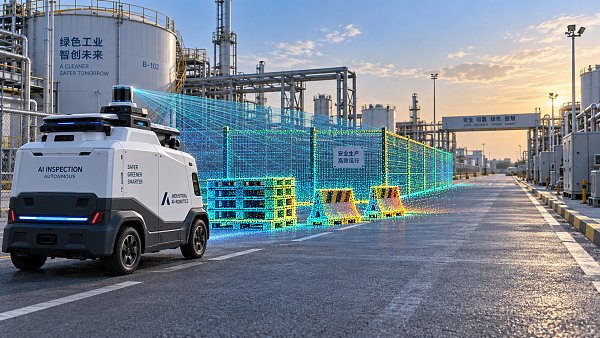
AGV and AMR systems add another layer. An agv traffic control algorithm may be computationally simple, yet latency increases if path updates, map sync, video feeds, and fleet coordination all traverse the same backhaul. For facilities with 10–50 mobile units, the control architecture matters as much as the onboard model. Local autonomy can absorb network fluctuation; centralized control can magnify it.

Typical bottlenecks by layer

The table below summarizes where industrial edge latency usually accumulates and what teams should verify before issuing RFQs or technical approval requests.

The key takeaway is simple: low inference time does not guarantee low decision latency. Teams should request per-stage timing logs, not one averaged number. TSV’s engineering view is to benchmark the chain at the interfaces, because that is where hidden delay usually appears.

What changes when 5G industrial routers are added?

A 5g industrial router throughput test is useful, but throughput alone is not enough. Industrial traffic includes small control packets, burst telemetry, image uploads, and periodic management traffic. A router that looks strong in peak bandwidth may still perform poorly in jitter-sensitive control if uplink scheduling, VPN overhead, or packet prioritization is not tuned for mixed traffic.

For remote assets, mobile robotics, and temporary lines, 5G can shorten deployment cycles from several weeks to a few days. Yet its value depends on architecture. If AI inference remains local and only summarized events travel over 5G, latency is often manageable. If raw streams are sent upstream for inference, the dependency on radio conditions increases sharply. That is a design choice, not a marketing feature.

How different industrial scenarios change acceptable latency thresholds

Not every plant needs the same edge response. A pass/fail inspection station, a high-speed packaging line, a UAV ground control node, and an AGV dispatch system operate under different timing economics. Good system design starts by matching latency tolerance to operational consequences: scrap, safety margin, throughput loss, operator intervention, or mission failure.

In robotics and automation, line takt time is often the anchor metric. If a station cycles every 2–5 seconds, an AI decision loop of 100–200 ms may be acceptable. But if the application is collision avoidance or dynamic grasp correction, the decision window may be much tighter. For AGV traffic control algorithm tuning, the relationship between vehicle speed and control update frequency should always be reviewed together.

In sensors and edge AI deployments, image size and object density strongly affect performance. A 640×480 stream and a 1920×1080 stream may use the same model family but create very different decode and preprocessing delays. Teams should not compare vendor demos unless camera configuration, illumination, compression, and output protocol are aligned.

In UAV and aerospace support workflows, latency is not only about speed but also about predictability. A stable 80 ms is often easier to integrate than a 30 ms average with 200 ms spikes. That is why jitter, worst-case delay, and failover behavior should be part of any technical review for mission-sensitive edge systems.

Scenario-oriented latency guidance

The following comparison helps information researchers, operators, buyers, and enterprise leaders frame realistic requirements before contacting suppliers or approving pilot scope.

These ranges are not universal guarantees, but they provide a grounded starting point. The more safety-critical or throughput-sensitive the workflow, the more teams should focus on worst-case performance instead of average latency.

Three signs your latency target is set too loosely

• Operators need frequent manual overrides during peak shifts, even though pilot tests looked stable.
• The system meets average timing in reports but shows burst delays during line changeovers, alarm storms, or simultaneous uploads.
• Procurement accepted chip-level benchmarks, but no one specified sensor-to-action timing, queue policy, or response under multi-client OPC UA sessions.

When these symptoms appear, the remedy is usually architectural: smaller payloads, local filtering, better traffic segmentation, or clearer division between local autonomy and central coordination.

What should buyers and engineers check before selecting an edge AI platform?

A useful procurement process separates lab capability from production readiness. Buyers should ask not only “How fast is the model?” but also “What is the full latency path under our protocol stack, our image size, our ambient temperature, and our concurrency level?” That single shift in wording often reveals whether a vendor understands industrial execution or only demo conditions.

For edge ai inference latency industrial projects, the best RFQs typically include 5 categories: sensor configuration, data transport design, protocol behavior, compute environment, and control integration. If even one category is omitted, the response may look attractive but remain non-comparable across suppliers. Decision-makers should insist on test conditions that can be repeated during FAT, SAT, or pilot acceptance.

TSV’s position is especially relevant here. In a market full of broad claims, engineering teams need a commercial filter that turns vague performance statements into measurable checkpoints. That is where independent benchmarking, parameter traceability, and full-path validation help reduce supplier qualification cycles and trial-and-error cost.

A disciplined evaluation also protects operations teams. If thermal throttling appears after 2–4 hours, or message queues back up during shift changes, operators will pay the price long after procurement signs off. Therefore, the acceptance checklist should include sustained-run timing, not just startup benchmarks.

A practical 6-point evaluation checklist

1. Define one end-to-end KPI, such as sensor-to-alert, camera-to-reject, or event-to-stop. Keep it measurable and tied to the actual workflow.
2. Request per-stage timing: acquisition, transmission, preprocessing, inference, postprocessing, and output. Avoid one-number summaries.
3. Test realistic payloads. Validate mqtt broker payload size limit policy and confirm what happens when messages exceed expected ranges.
4. Measure integration timing. Ask for opc ua server response time with production-like tag density, not a small demo namespace.
5. Run sustained tests for 8–24 hours. Watch for heat, queue growth, dropped frames, and control delay spikes.
6. Validate failover behavior. If the backhaul degrades or a broker restarts, confirm the local edge node still handles critical logic safely.

This checklist improves comparison quality across vendors, system integrators, and internal teams. It also gives procurement a defensible structure for approvals, because every item links to measurable operational risk.

Common sourcing misconceptions

“Higher TOPS always means lower latency”

Not necessarily. If decode, transport, or protocol handling dominate the chain, more accelerator power may provide little practical benefit. Hardware sizing must match the real bottleneck.

“Cloud fallback solves everything”

Cloud resources help analytics, fleet overview, and model management, but critical industrial control loops usually need local decision capability. Backhaul variability can be tolerated for reporting; it is much harder to tolerate for immediate machine action.

“Average latency is enough for qualification”

Production systems fail on spikes, not averages. Always ask for percentile behavior, worst-case observations, and test context such as simultaneous streams, mixed traffic, and uptime duration.

How to implement a lower-latency architecture without overbuying hardware

Reducing edge latency does not always mean buying the most expensive platform. In many projects, the first gains come from architecture: moving preprocessing closer to the sensor, shrinking payloads, separating control traffic from bulk data, and keeping time-critical decisions local. This is especially true when budget pressure and short deployment windows force teams to prioritize return on engineering effort.

For example, if MQTT is used for event distribution, push metadata and exception snapshots rather than continuous raw images. If OPC UA is used for machine integration, define a narrow command set for time-critical actions and avoid unnecessary tag chatter. If 5G is used, reserve it for mobility or remote access while preserving local fallback logic on the edge node. These steps often reduce both latency and bandwidth cost.

Another cost lever is model-system alignment. A smaller optimized model running inside a disciplined pipeline can outperform a larger model trapped in inefficient transport and conversion layers. For many industrial tasks, consistency across 8-hour, 16-hour, or 24-hour operation matters more than peak benchmark figures measured for a few minutes.

Implementation should also follow a staged process. Most facilities benefit from a 3-stage rollout: bench validation, pilot under production traffic, and limited-scale production acceptance. Each stage should have explicit timing criteria, rollback conditions, and interface responsibility. This lowers both technical risk and procurement ambiguity.

A lean implementation path

• Stage 1, bench test in 7–15 days: confirm per-stage timing, thermal behavior, and interface compatibility with actual sensors and protocols.
• Stage 2, pilot in 2–4 weeks: run the system on one line, one zone, or a limited AGV cluster under normal shift conditions and changeover events.
• Stage 3, controlled scale-up: expand only after validating message stability, operator workflow, failover logic, and KPI repeatability across multiple cycles.

This approach helps enterprises avoid the common trap of buying for theoretical maximum load before they understand the real operational bottleneck. It is more efficient to eliminate wasted transport and protocol overhead first, then right-size compute hardware.

FAQ: the questions industrial teams ask before approval

How do we evaluate edge AI latency if vendors provide only model FPS?

Ask for an end-to-end timing breakdown under your intended workflow. At minimum, request acquisition time, network or middleware delay, preprocessing time, inference time, and command output time. If possible, require a sustained 8–24 hour test and include real payload sizes, actual camera settings, and expected protocol concurrency.

What payload strategy is safer for MQTT in industrial edge systems?

Use MQTT mainly for lightweight telemetry, event status, and references to larger data objects. Avoid pushing oversized images or verbose serialized content through the broker unless the architecture is explicitly designed for it. Confirm mqtt broker payload size limit settings and test what happens during retry bursts or broker restarts.

How important is OPC UA timing for edge AI projects?

It is critical whenever AI output drives machine behavior, alarms, or process routing. The opc ua server response time should be measured with realistic namespace size, tag subscription counts, and concurrent clients. A clean demo server often hides delays that appear once MES, SCADA, and local HMIs connect together.

When does a 5G industrial router make sense?

It is most useful for mobile assets, remote facilities, temporary production layouts, and sites where wired backhaul is slow to deploy. But the 5g industrial router throughput test should include mixed traffic, VPN overhead, and event bursts. It is a strong transport option, not a substitute for sound local edge architecture.

Why choose TSV when latency claims need engineering proof

TechStat Vanguard is built for teams that need parameters, not adjectives. In hard-tech procurement and system evaluation, the real question is not whether a platform sounds advanced, but whether its timing, tolerance, and integration behavior hold up under industrial conditions. TSV helps engineering teams, buyers, and executives separate benchmark reality from presentation-layer claims.

Our value is strongest when projects cross disciplines: sensors, edge AI, industrial networking, automation logic, and supply-chain sourcing. We focus on measurable evidence such as latency paths, throughput constraints, protocol behavior, and deployment trade-offs. That makes our analysis useful for spec sheet drafting, supplier comparison, and pilot gate reviews.

If you are reviewing an edge AI system, you can contact TSV to discuss parameter confirmation, latency path decomposition, product selection logic, protocol stack impact, expected delivery windows, custom evaluation criteria, and practical trade-offs between local processing and backhaul dependency. We can also help structure technical questions for vendors so that quotations and demos become comparable.

For enterprises facing short qualification cycles, mixed vendor claims, or uncertainty around agv traffic control algorithm timing, mqtt broker payload size limit, opc ua server response time, or 5g industrial router throughput test results, a data-driven review reduces risk before budget is committed. In industrial edge AI, the fastest model is not always the fastest system. The system that wins is the one engineered around the full path.