AGV traffic control algorithm bottlenecks at intersections

In high-throughput warehouses, the real challenge is not vehicle speed but how an agv traffic control algorithm handles intersection conflicts, deadlocks, and priority rules under live demand. For engineers, operators, buyers, and decision-makers, understanding these bottlenecks is essential to improving warehouse management system wms integration, fleet efficiency, and measurable automation reliability.

Intersection control is where many AGV projects either prove their maturity or expose hidden architectural weaknesses. A fleet may run smoothly at 5 to 10 vehicles, yet show congestion, path oscillation, or repeated stop-and-go behavior when scaled to 30, 50, or 100 units. At that point, the limiting factor is not traction motor performance or battery capacity, but scheduling logic, communication latency, and rule design.

For TSV’s target audience, this topic matters for different reasons. Engineers care about deterministic dispatch, conflict resolution, and recovery time. Operators care about missed picks, blocked aisles, and unsafe waiting behavior. Procurement teams need a practical way to compare supplier claims. Business leaders need to know whether a traffic control stack will support growth without forcing expensive retrofits in 12 to 24 months.

A credible evaluation of AGV intersection performance should therefore focus on hard operational signals: queue length, waiting time per node, deadlock recovery cycle, route recalculation frequency, WMS/WCS handshake speed, and throughput loss under peak order bursts. These are the metrics that separate a marketable demo from an industrial system that can run three shifts a day.

Why intersections become the core bottleneck in AGV fleet control

An AGV traffic control algorithm usually performs well in linear routes, low-density loops, or fixed sequencing tasks. The problem emerges at shared nodes where multiple vehicles request the same physical space within a short time window. In a warehouse with 4-way crossings, narrow transfer lanes, and mixed-priority missions, one poorly tuned intersection can reduce effective fleet throughput by 15% to 35% even when the vehicles themselves are healthy.

The first constraint is spatial exclusivity. A vehicle cannot partially reserve a crossing and assume that another unit will yield correctly under all cases. If the control layer allows ambiguous reservation zones, AGVs may hesitate, stop in buffer areas, or enter a conflict region too early. This creates ripple effects: delayed pallet moves, blocked replenishment routes, and idle time at picking stations that are otherwise fully staffed.

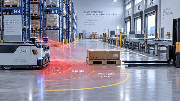
The second constraint is timing uncertainty. Even a 100 to 300 millisecond communication delay can matter when several AGVs approach the same node at 1.2 to 2.0 m/s. If the controller updates route permissions too slowly, the fleet begins to behave conservatively, increasing stop frequency and lowering path efficiency. If it updates too aggressively without safe state validation, the system raises collision risk or produces unstable rerouting loops.

The third issue is rule conflict between local and global optimization. A local rule may reduce waiting time at one intersection, while worsening congestion across the whole plant. For example, always giving priority to loaded vehicles sounds reasonable, but in some layouts it starves return-empty traffic and creates accumulation at charging or staging zones. Over a full shift, that imbalance can increase cycle time by 8% to 20%.

Typical sources of intersection inefficiency

• Static priority rules that do not adapt to real-time queue length or mission urgency.
• Oversimplified map zoning, where one logical node represents too large a physical area.
• Slow WMS or WCS feedback, causing dispatch orders to arrive after routing windows have changed.
• Insufficient buffer design near workstations, leading AGVs to wait inside active transport lanes.
• Poor exception handling when one vehicle stops unexpectedly for obstacle avoidance or battery protection.

What decision-makers should measure first

Before changing hardware or adding more vehicles, teams should establish a baseline using 5 core indicators: average node waiting time, 95th percentile waiting time, deadlock frequency per shift, route recalculation count per hour, and completed missions per hour. These indicators reveal whether the problem is algorithmic, architectural, or operational.

Main algorithm bottlenecks: reservation logic, deadlock handling, and priority design

Most intersection failures can be traced to three layers of logic: path reservation, deadlock prevention and recovery, and mission priority assignment. Each layer may look acceptable during factory acceptance testing with 10 to 20 scenarios, but warehouses rarely operate in such a controlled state. Real demand introduces uneven task release, manual interruptions, battery returns, and temporary aisle occupation that expose weak control assumptions within hours.

Reservation logic determines how much road segment an AGV can lock ahead of movement. If reservations are too short, the fleet stops frequently and throughput drops. If reservations are too long, vehicles occupy unnecessary space and trigger artificial scarcity. In practice, many sites perform best when reservation windows are segmented by approach zone, crossing zone, and exit zone rather than using a single coarse block.

Deadlock handling is often misunderstood. Some suppliers claim deadlock-free design, but that statement only holds under specific map topology and rule assumptions. In mixed traffic networks, temporary deadlocks and near-deadlocks can still occur when AGVs reserve opposing lanes, wait on battery-related restrictions, or react differently to obstacle sensor events. The key is not pretending deadlocks never happen, but limiting detection time and recovery cost.

Priority design is another frequent blind spot. A purely first-come-first-served model is predictable but may penalize urgent replenishment tasks. A strongly weighted priority model can favor high-value orders but create starvation for low-priority missions. Robust systems use bounded priority rules, aging mechanisms, and exception overrides so that a task delayed for 90 to 180 seconds eventually rises in dispatch rank.

Comparison of common control approaches at intersections

The table below compares typical AGV traffic control approaches used in warehouses and manufacturing logistics. It highlights where each method tends to fail when intersection density increases.

For most B2B users, the practical answer is not choosing the most advanced algorithm on paper, but the one that remains stable under live order variability, temporary congestion, and integration delays. A modestly optimized but observable system usually outperforms a complex controller that operators cannot diagnose.

Common deadlock recovery methods

1. Timeout-based rollback after 10 to 30 seconds of no forward progress.
2. Reverse-release logic to free one reserved segment and allow path reordering.
3. Dispatcher override using mission criticality, battery state, and workstation dependency.
4. Temporary one-way corridor enforcement during peak periods or abnormal congestion.

Integration limits: how WMS, WCS, and edge communication shape traffic outcomes

Even a well-designed agv traffic control algorithm cannot deliver strong intersection performance if upstream and downstream systems exchange data too slowly or inconsistently. In practice, AGV control is deeply coupled with WMS task release, WCS orchestration rules, scanner events, conveyor handshakes, and battery management logic. When one of these layers lags, intersections become the visible symptom of a wider digital coordination problem.

A common issue is asynchronous task timing. The WMS may release replenishment missions in large bursts every 30 or 60 seconds, while the AGV fleet controller expects smoother dispatch intervals. This bursty pattern floods a few shared nodes at the same time. Instead of distributing missions over a 2 to 5 minute window, the system creates micro-congestion waves that repeatedly overload the same intersections.

Another limitation is telemetry freshness. If location, mission status, or zone occupancy data is delayed by more than 200 to 500 milliseconds in a dense environment, the controller starts making decisions on stale information. The result is unnecessary yielding, duplicate route calculations, and missed opportunities to use small time gaps safely. In high-value operations, this can translate into lower pick rate consistency and avoidable overtime costs.

Edge computing can help, but only when responsibility boundaries are clear. Local controllers may handle immediate node arbitration faster than a fully centralized cloud-dependent stack. However, if local logic and central optimization disagree about mission priority or corridor locking, the site experiences unstable behavior. The architecture must define which layer controls intersection permission, rerouting authority, and exception recovery.

Key integration checkpoints before scaling fleet size

The following table helps engineering and procurement teams verify whether traffic bottlenecks come from algorithm design or system integration quality.

If these checkpoints are not controlled, buying a new fleet controller may not solve the actual bottleneck. The more reliable path is to benchmark interface timing, node occupancy logic, and mission release behavior before blaming vehicle hardware or adding more AGVs.

Integration warning signs operators should not ignore

• Intersections clogging only during ERP-driven order waves, not during manual test runs.
• AGVs stopping near handoff equipment even though no physical obstacle is present.
• Frequent rerouting after battery state changes or charger requests.
• Different waiting behavior between day shift and night shift because task mix changes.

Selection criteria for buyers and technical teams evaluating AGV traffic control

From a procurement perspective, the biggest mistake is evaluating AGV systems by top speed, nominal payload, or interface count alone. These are necessary specifications, but they do not prove that an agv traffic control algorithm can sustain stable throughput at busy intersections. A more defensible buying process compares operational behavior under density, exception load, and integration complexity.

Request suppliers to demonstrate traffic performance in at least 3 scenarios: normal load, peak load, and disturbed load. Disturbed load should include one blocked node, one delayed handoff, and one priority task injection. If a vendor can only show ideal path following, the risk is that your site becomes the real test environment after commissioning. For capital equipment projects, that risk is usually far more expensive than a higher upfront software evaluation effort.

It is also important to distinguish AGV and AMR claims carefully. Some autonomous systems can navigate around local obstacles well, but still rely on simplified fleet arbitration at shared intersections. Good local autonomy does not automatically equal strong multi-vehicle traffic governance. Buyers should ask where intersection authority lives, how node locking is handled, and how the system resolves conflicting missions within 5, 10, and 30 second windows.

Technical due diligence should include observability. Can the supplier expose intersection wait logs, queue heat maps, and deadlock incident traces? Can engineers change priority parameters without rewriting the entire logic tree? Can operators identify whether a delay came from WMS task release, traffic reservation, or workstation handshake failure? If not, troubleshooting after go-live becomes slow and politically difficult.

A practical procurement checklist

1. Validate fleet size range already proven in layouts with comparable intersection density.
2. Ask for queue time visibility at node level, not only aggregate mission completion data.
3. Review deadlock detection and recovery sequence, including timeout values and operator override.
4. Confirm whether priority logic supports aging, urgent task insertion, and charging exceptions.
5. Check integration ownership across WMS, WCS, PLC, and fleet control before contract finalization.
6. Define acceptance tests using measurable thresholds such as less than 5% mission delay above target during peak simulation.

Questions worth asking suppliers

Ask how the system behaves when 20% of missions are urgent, when one charging station is unavailable, or when a high-traffic node is blocked for 3 minutes. Ask whether the supplier can simulate 1.5x expected future volume rather than only current demand. This matters because many warehouses change SKU mix, shift pattern, and replenishment frequency within 6 to 18 months after automation launch.

For executive teams, a useful benchmark is scalability without redesign. If a control architecture supports only today’s map and traffic logic, expansion becomes costly. A system that can absorb another 25% to 40% task volume through rule tuning and buffer redesign has much stronger lifecycle value.

Implementation, tuning, and continuous optimization in live operations

Commissioning should not end with route validation and basic collision avoidance testing. The real work begins when the AGV traffic control algorithm is tuned under production rhythm. A structured rollout usually has 3 stages: baseline mapping and reservation setup, peak-load simulation with exception injection, and live optimization after 2 to 4 weeks of actual operation data. Skipping the third stage leaves valuable performance gains unrealized.

During tuning, teams should identify the 10 to 20 highest-delay nodes and classify root causes. Some nodes fail because the reservation zone is too large. Others fail because handoff equipment releases slowly, or because nearby charging requests disrupt path symmetry. By separating algorithmic issues from layout and process issues, the site can avoid repeated software changes that do not address the real constraint.

Continuous optimization depends on disciplined data review. Weekly dashboards should track at least 6 metrics: missions completed per hour, average and 95th percentile intersection waiting time, deadlock events, forced reroutes, battery-related path disruptions, and workstation service delay. Over 8 to 12 weeks, these indicators show whether operational changes are stabilizing the fleet or merely shifting congestion from one area to another.

TSV’s engineering perspective is straightforward: parameters matter more than marketing language. If a supplier cannot show how priority thresholds, timeout settings, zone segmentation, and interface timing affect throughput, the traffic control layer is not yet transparent enough for serious industrial comparison. Precision in logic design, not sales adjectives, is what reduces trial-and-error cost.

Recommended post-go-live improvement cycle

• Week 1–2: confirm map accuracy, node occupancy states, and stop-position consistency.
• Week 3–4: compare planned versus actual queue time at the top 10 intersections.
• Month 2: tune reservation length, aging rules, and charger dispatch thresholds.
• Month 3: run a controlled stress test at 120% of normal mission rate if operations allow.
• Quarterly: review whether WMS release strategy still matches current SKU and order profile.

FAQ: what teams ask most often

How many AGVs usually trigger intersection problems? There is no universal threshold, but many sites first notice instability between 15 and 40 vehicles, depending on map density, aisle width, and mission overlap.

Can more intersections solve the issue? Sometimes, but not always. Adding paths without redesigning priority and reservation logic may simply distribute congestion differently. Physical layout and control policy must be evaluated together.

Is deadlock always a software fault? Not entirely. Software is central, but deadlocks can also reflect poor buffer placement, delayed equipment handoff, and charger positioning that forces unnecessary crossing traffic.

Should buyers demand simulation results? Yes. A credible simulation should cover normal load, peak load, and exception scenarios, and it should show measurable outputs such as waiting time, queue length, and mission completion rate rather than only animated vehicle movement.

For warehouses pursuing scalable automation, intersection control is the real proving ground of fleet intelligence. The strongest systems are not the ones with the most dramatic claims, but the ones that can show stable queue behavior, fast deadlock recovery, transparent priority rules, and disciplined WMS/WCS integration under live demand.

If your team is comparing AGV suppliers, refining warehouse traffic logic, or preparing a technical specification for a new project, a data-driven review of intersection behavior will save time, reduce qualification risk, and improve long-term automation value. Contact TSV to discuss benchmarking priorities, evaluate control architecture, or explore a more precise framework for AGV traffic performance assessment.