Vision based quality inspection software in low contrast scenes

In low-contrast production environments, vision based quality inspection software must do more than detect defects—it must deliver stable accuracy, fast processing, and actionable data for engineering and procurement teams alike. This article explores how advanced machine vision software, edge AI inference latency industrial factors, and industrial IoT dashboard visualization shape reliable inspection performance in demanding manufacturing scenarios.

For R&D teams, the central question is not whether a vision system can identify a flaw under ideal lab lighting, but whether it can maintain repeatable inspection results across 8-hour, 16-hour, or even 24/7 production cycles. For operators, stability and usability matter as much as model accuracy. For procurement leaders and decision-makers, the focus shifts to measurable output: false reject rate, missed defect rate, deployment time, maintenance burden, and integration cost.

Low-contrast scenes are common in electronics assembly, precision machining, composite materials, medical consumables, aerospace subcomponents, and reflective packaging lines. In these environments, small scratches, shallow dents, incomplete fills, subtle print shifts, or edge burrs may differ from the background by only a few grayscale levels. That narrow visual margin changes how software should be selected, benchmarked, and deployed.

Why low-contrast inspection is a separate engineering problem

Low-contrast inspection is often underestimated because many proof-of-concept trials are performed under controlled conditions. On the factory floor, contrast can vary due to oil film, surface oxidation, ambient light leakage, part orientation, vibration, and lens contamination. A defect that appears visible at 4:1 contrast in the lab may drop below 1.5:1 during live production, where conventional threshold-based algorithms begin to fail.

This is why vision based quality inspection software in low contrast scenes must be engineered as a system, not purchased as a feature checklist. Image acquisition, preprocessing, model training, edge inference, and dashboard feedback are linked. If one element is weak, overall inspection consistency drops. In many lines, a 1% increase in false rejects can create unnecessary scrap, operator rework, and line stoppage within days.

The software layer becomes especially important when the optical setup cannot be changed easily. Some lines have fixed mechanical space, short cycle times of 200–800 ms per part, and existing PLC logic that leaves limited room for hardware redesign. In these cases, software must compensate for contrast instability through adaptive enhancement, region-based analysis, and defect classification logic that remains explainable to engineering teams.

Typical failure modes in low-contrast scenes

Several failure modes appear repeatedly across industries. The first is low signal separation, where the grayscale or color difference between good and defective surfaces is too small for static rules. The second is background drift, where lighting or material finish changes over a production batch of 500 to 5,000 parts. The third is annotation inconsistency, where human labeling of subtle defects differs from shift to shift, weakening supervised model training.

• Micro-scratches on polished metal where defect depth is visible only under directional illumination.
• Incomplete adhesive spread where the edge boundary is blurred and changes with substrate absorption.
• Shallow dents or sink marks on molded parts with less than 3–5 grayscale levels of difference.
• Faint print contrast changes on labels, foils, or pharmaceutical blister packaging.

These issues explain why buyers should request sample-based evaluation under real process conditions rather than relying on vendor screenshots. At minimum, benchmarking should include 3 defect classes, 2 lighting conditions, and 1 full production batch review to establish realistic performance boundaries.

What engineering teams should measure first

Before discussing AI architecture, teams should define the inspection target. That means specifying defect size, defect contrast, allowed escape rate, allowed false reject rate, and cycle time. A low-contrast scratch that is 0.2 mm wide and 3 mm long is a different problem from a 1.5 mm stain with variable tone. Without these thresholds, software selection becomes subjective and procurement comparisons become unreliable.

A practical review framework is shown below. It helps align engineering, quality, operations, and sourcing teams around measurable acceptance criteria rather than marketing language.

The key takeaway is simple: low-contrast inspection cannot be evaluated on accuracy alone. It must be judged through a combined lens of detectability, speed, stability, and operational cost. Teams that quantify these four dimensions early usually shorten supplier qualification cycles by several weeks.

Core software capabilities that improve detection reliability

The best machine vision software for low-contrast scenes combines deterministic image processing with data-driven learning. Pure rule-based pipelines often struggle when contrast shifts across lots, while pure deep learning approaches may become opaque and data-hungry. A hybrid design usually performs better in industrial settings because it uses controlled preprocessing to normalize images before classification or segmentation.

At the preprocessing level, useful functions include local contrast enhancement, background flattening, glare suppression, denoising, and sub-pixel edge extraction. At the model level, the software should support defect classification, anomaly detection, and pixel-level segmentation. In practice, anomaly detection is often valuable when defect appearance is variable but good parts are abundant, while segmentation is more suitable when defect boundaries must be measured or traced.

Another critical capability is explainability. Engineering teams need to know why the software rejected a part, especially when the defect is subtle. Heatmaps, region overlays, score histograms, and defect confidence thresholds help teams tune sensitivity. If software only outputs pass or fail with no traceable evidence, it becomes difficult to validate during FAT, SAT, and ongoing quality audits.

Preferred technical functions for challenging surfaces

In low-contrast conditions, several software functions have above-average value. Not every line needs all of them, but they should be considered during technical review:

1. Adaptive ROI processing to focus compute resources on critical zones instead of full-frame analysis.
2. Multi-exposure or image fusion support when one exposure cannot separate background and defect simultaneously.
3. Version-controlled recipe management for 5 to 50 product variants on the same line.
4. Confidence threshold tuning with reject bin analysis over at least 1,000 sample parts.
5. Operator-assisted relabeling workflows for continuous model improvement without full engineering intervention.

These functions matter because low-contrast defects rarely remain visually stable over time. Surface finish can drift gradually, and acceptable thresholds may change by customer, plant, or product generation. Software should therefore support controlled adaptation without introducing uncontrolled model drift.

Balancing sensitivity and over-rejection

A common mistake is pushing the model for maximum sensitivity during trials. That may catch more subtle defects, but it can also raise false rejects from 0.8% to 4% or more when process variation increases. In real production, excessive over-rejection often costs more than the defect class the system was meant to catch. The better approach is to define acceptance bands, validate them over multiple shifts, and align them with actual downstream risk.

For example, if a cosmetic scratch has no effect on function but triggers customer complaints only above a visible size threshold, the software should be tuned to that threshold rather than to every detectable imperfection. Good vision based quality inspection software supports this calibration at recipe level, making it easier to align inspection policy with business reality.

Edge AI inference latency industrial factors and line performance

Even highly accurate inspection models can fail operationally if edge deployment is slow or unstable. Edge AI inference latency industrial factors include processor selection, image size, model complexity, network overhead, PLC handshake timing, and the number of inspection tasks running in parallel. On a line producing 60 to 300 parts per minute, an additional 150 ms delay can become a real throughput issue.

Latency must be assessed end to end, not just at model inference level. A model may process in 35 ms on a benchmark device, but full cycle time can still exceed 180 ms after image transfer, pre-processing, result formatting, trigger buffering, and MES reporting. Procurement teams should therefore request measured line-side timings instead of isolated GPU or CPU claims.

There is also a reliability dimension. Edge platforms deployed in industrial cabinets may operate at 35°C to 45°C ambient temperature, with dust, vibration, and power noise. A software stack that performs well in development can degrade if thermal throttling begins after several hours. Stable industrial inspection requires not only fast inference but also predictable inference over time.

What to benchmark during pilot projects

A strong pilot plan should measure at least four timing layers: image acquisition time, preprocessing time, model inference time, and result transmission time. It should also test warm-state performance after 2–4 hours of continuous operation. If your cycle target is 500 ms, a safe engineering rule is to keep average total processing below 300 ms and peak processing below 400 ms to preserve operational margin.

The table below can be used as a practical benchmark structure during supplier comparison or internal evaluation.

The main conclusion is that edge AI performance should be purchased as a production metric, not a component metric. For many manufacturers, a predictable 80 ms inference with stable thermal behavior is more valuable than a claimed 25 ms benchmark that cannot be sustained over a full shift.

Deployment choices that affect throughput

Single-station deployments are simpler, but many factories need one edge node to serve 2–4 cameras or several inspection tasks. That changes CPU load, GPU memory usage, and scheduling behavior. Buyers should ask whether performance has been validated under multi-stream conditions. They should also clarify if software updates require line downtime of 30 minutes, 2 hours, or an entire shift.

• Use hardware profiles matched to image resolution and expected camera count.
• Reserve at least 20% processing headroom for batch variation and future recipe expansion.
• Validate restart recovery time after power loss; practical targets are often under 3–5 minutes.
• Confirm local buffering if network loss lasts 10–30 seconds during MES communication.

Industrial IoT dashboard visualization and closed-loop quality control

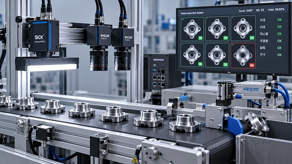
Inspection is more valuable when results are visible, traceable, and actionable. Industrial IoT dashboard visualization connects vision based quality inspection software to broader plant intelligence. Instead of only reporting pass or fail, a useful dashboard shows defect type distribution, reject trends by shift, camera health, model confidence drift, and recipe-level performance. This allows teams to separate actual process deterioration from inspection instability.

For operators, dashboards should reduce ambiguity. A well-designed interface highlights the top 3–5 defect categories, displays annotated images, and flags whether a spike is localized to one station or spread across the line. For quality engineers, historical trend views over 24 hours, 7 days, and 30 days support root-cause analysis. For procurement and management, dashboards provide evidence of utilization, downtime drivers, and payback progress.

This visibility becomes especially important in low-contrast applications because software thresholds may need tuning over time. If contrast drift is caused by upstream process changes, such as tool wear, coating thickness deviation, or lighting degradation, the dashboard can reveal pattern shifts before scrap escalates. The inspection system then becomes part of process control, not just final gatekeeping.

Dashboard elements that create operational value

A practical industrial dashboard should not be overloaded. The most useful metrics are those that connect inspection performance to engineering actions and production decisions.

• Defect Pareto by station, product code, and shift over the last 8, 24, and 168 hours.
• False reject review queue with image evidence and operator disposition tags.
• Model confidence trendline to detect gradual drift in low-contrast discrimination.
• Camera, light, and edge device status for maintenance intervention before failure occurs.
• Batch traceability linked to lot number, timestamp, and recipe version.

When these metrics are visible, engineering teams can correlate inspection outputs with upstream machine parameters. For example, a rise in faint edge defects after 1.2 million machine cycles may indicate tool wear rather than software misclassification. That distinction is commercially important because it changes whether the fix belongs to maintenance, process engineering, or software tuning.

Data retention and governance considerations

Factories should also define how much data to keep. Full image storage for every part may be unnecessary and expensive, especially at 2–10 MB per image. A tiered policy often works better: retain defect images for 90–180 days, keep sampled good-part images for model validation, and store aggregated metrics for longer periods. This balances traceability with practical storage cost.

For regulated or high-liability sectors, access control and audit logs matter as much as visualization. Any adjustment to thresholds, recipes, or defect classes should be timestamped and attributable. That protects both manufacturers and suppliers during customer review, supplier qualification, and quality disputes.

How to select, validate, and procure the right inspection software

Selecting vision based quality inspection software in low contrast scenes should be treated as a cross-functional sourcing project. Engineering defines defect physics and acceptance thresholds. Operations defines takt time and usability constraints. IT or automation teams define integration boundaries. Procurement translates these into comparable commercial requirements. When one of these groups is excluded, the result is often a technically promising pilot that does not scale.

A good procurement process typically unfolds in 4 stages: requirement definition, sample validation, pilot deployment, and line-scale acceptance. Each stage should have explicit pass criteria. For example, stage 2 may require validation on 1,000 to 3,000 labeled images or on a live batch covering all known defect classes. Stage 3 may require one full week of line-side operation with downtime and false reject tracking.

Commercial evaluation should go beyond license price. Buyers should compare implementation scope, retraining support, recipe change effort, edge hardware requirements, dashboard functionality, and support response windows. In many cases, the lowest initial quote becomes the highest total cost if recipe maintenance or integration work is underestimated.

A practical vendor comparison matrix

The following matrix helps structure supplier discussions around objective criteria rather than claims of being “smart” or “advanced.”

The strongest candidates are usually those that combine measurable low-contrast performance with maintainable operations. A system that saves 2 seconds of engineering time per part review or reduces false rejects from 3% to 1% can produce meaningful annual value, even if its upfront price is not the lowest.

Common mistakes during selection

Three mistakes appear frequently. First, teams validate only curated defect images instead of actual production variation. Second, they compare model accuracy without comparing cycle time and maintenance effort. Third, they overlook dashboard and traceability requirements until after installation. These gaps tend to delay acceptance and create disputes between users, engineering, and vendors.

A disciplined selection process should include documented samples, clear defect definitions, acceptance metrics, and change-control rules. That is consistent with TSV’s engineering-first view: parameters, thresholds, and operating limits should be explicit from the beginning.

Implementation roadmap, risk control, and FAQ

Successful deployment usually follows a staged implementation path rather than a single installation event. A common roadmap includes 5 steps: line survey, image dataset collection, pilot model tuning, edge integration, and acceptance monitoring. Depending on line complexity, this can take 2–6 weeks for a focused station or 6–12 weeks for a multi-camera line with MES connectivity.

Risk control should be built into each phase. During dataset collection, teams should capture shifts, lots, and known contrast variations. During pilot testing, they should separate training, validation, and holdout samples. During live deployment, they should run the software in shadow mode before enabling automatic reject actions. This reduces the chance of unexpected over-rejection on day one.

Post-launch review is equally important. In the first 30 days, engineering teams should monitor top reject reasons, confidence drift, camera cleanliness, and operator override patterns. If the system requires frequent manual intervention, the issue may lie in workflow design rather than model quality alone.

FAQ: How do we know if low-contrast AI inspection is necessary?

If your defects vary in appearance, the contrast ratio is low, or rule-based tuning changes frequently between batches, AI-assisted inspection is worth evaluating. A practical signal is when traditional tools require repeated threshold adjustment more than once per shift or when review disputes between operators and quality staff become common.

FAQ: What sample size is reasonable for evaluation?

For an early feasibility test, a few hundred images may be enough. For a credible pilot, many teams target 1,000–3,000 labeled images or a representative live batch that covers good parts and all major defect classes. The right number depends on defect diversity and whether anomaly detection or supervised classification is used.

FAQ: How long does deployment usually take?

A simple single-station project can move from survey to live validation in 2–4 weeks if optics and interfaces already exist. More complex lines with PLC, MES, and dashboard integration often need 6–10 weeks, especially when acceptance criteria and traceability requirements are strict.

FAQ: Which KPIs should procurement request in contracts or technical agreements?

Useful KPIs include defect detection threshold, false reject ceiling, maximum end-to-end processing time, supported recipe count, uptime target, issue response time, and retraining support scope. Contract language should specify how these are measured, over what sample volume, and under which production conditions.

In low-contrast manufacturing scenes, the right inspection platform is one that turns subtle visual uncertainty into measurable process control. The most effective solutions combine robust machine vision software, realistic edge AI latency management, and industrial IoT dashboard visualization that engineering, operations, procurement, and management can all use. If your team is evaluating inspection stability, supplier capability, or deployment feasibility, now is the right time to define measurable thresholds and test them against real production data. Contact us to discuss your application, request a tailored evaluation framework, or explore a practical inspection roadmap for your line.