How to Reduce Quality Inspection Automation Response Time on High-Speed Lines

Why does quality inspection automation response time matter so much on fast lines?

On a high-speed line, delay is rarely visible to the eye. It appears as missed rejects, unstable sorting, or defects discovered too late.

That is why quality inspection automation response time deserves attention beyond pure throughput. It directly affects containment, traceability, and process discipline.

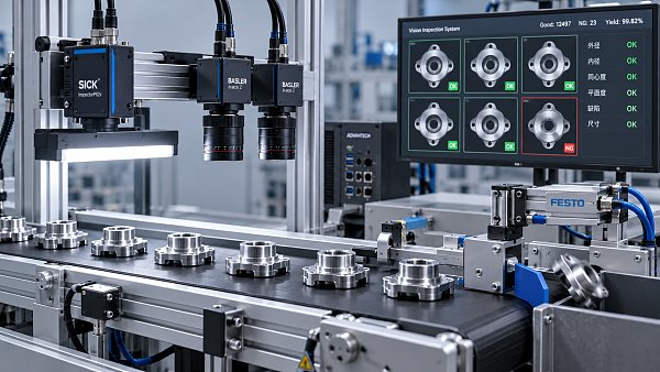
In practical terms, response time includes image capture, signal transfer, model inference, decision logic, actuator trigger, and confirmation feedback.

Many teams focus on camera resolution or robot speed first. More often, the real bottleneck sits between sensing and action.

A line can run at full nominal speed and still carry hidden latency. That latency raises the chance of defect escape into packaging, assembly, or shipment.

This is especially critical where safety, aerospace, electronics, medical components, or precision machining require strict tolerance control.

TechStat Vanguard often frames this issue in a simple way: parameters matter more than claims. If response time is not measured end to end, it is being guessed.

For that reason, improving quality inspection automation response time should start with engineering evidence, not supplier brochures or generic speed ratings.

Where is the delay actually coming from?

When response time is too slow, the problem is usually distributed across several layers rather than one dramatic failure point.

A useful first step is to split the inspection cycle into measurable segments. That prevents teams from blaming the vision system alone.

The most common latency sources include:

• Trigger instability from encoders, sensors, or inconsistent part spacing.
• Image exposure settings that trade blur reduction for slower acquisition.
• Large image files moving through overloaded industrial networks.
• Edge AI or rule-based software processing more data than the decision requires.
• PLC scan time, handshake delays, or poorly tuned reject mechanisms.
• Feedback loops that confirm reject success too late for corrective action.

In actual plants, a fast camera paired with a slow reject gate can still produce poor quality inspection automation response time.

The same applies to AI inspection. A highly accurate model may become unsuitable if inference time exceeds available line distance.

The table below helps isolate which symptom usually points to which bottleneck.

How can response time be reduced without sacrificing inspection accuracy?

This is the question that usually matters most. The answer is to shorten unnecessary processing, not to weaken inspection logic blindly.

A strong approach begins with the decision itself. Ask what signal is truly needed to accept, reject, or divert the part.

If a defect can be confirmed from one region, avoid full-frame analysis. If one threshold works, avoid layered logic that adds no control value.

In many systems, the fastest improvement comes from narrowing the region of interest and reducing image transfer load.

Lighting also deserves attention. Stable lighting lowers the need for heavy filtering, repeated captures, or model compensation.

Another effective move is shifting inference closer to the line. Edge processing often cuts network travel and server queue delays.

For systems using PLCs, logic simplification can be surprisingly valuable. Long decision trees and excessive handshakes add latency one scan at a time.

Mechanical response should be tuned with the same discipline as software. A precise camera cannot compensate for a slow pneumatic rejector.

• Reduce image size only after confirming defect visibility remains acceptable.
• Use deterministic industrial Ethernet where inspection timing is critical.
• Synchronize timestamps across camera, controller, and MES records.
• Measure actual reject success, not just software decision speed.

The best quality inspection automation response time usually comes from balanced tuning across optics, compute, controls, and motion.

When does faster inspection become risky?

Not every speed gain is a good gain. Some changes reduce latency while quietly weakening detection coverage or compliance evidence.

A common mistake is lowering image resolution too far. This may improve quality inspection automation response time while hiding small cracks, burrs, or contamination.

Another risk appears when teams skip result validation. Faster logic looks successful until false rejects rise or escaped defects appear downstream.

There is also a traceability risk. If systems remove buffering or logs to gain speed, root-cause analysis becomes harder after an incident.

This matters in regulated environments and in sectors where supplier qualification depends on hard evidence rather than verbal claims.

A more reliable method is to set a minimum detection capability first. Then optimize latency inside that boundary.

That principle aligns with the TSV view of engineering truth. Response time should be benchmarked against repeatability, tolerance, and verified defect capture performance.

If a faster setting cannot be defended with measured data, it is not really an improvement.

What should be checked before investing in new hardware or software?

Buying a faster camera or accelerator card can help, but only after the timing chain is understood.

In actual applications, upgrades deliver the best return when current limits are documented with numbers rather than assumptions.

Before selecting a new platform, confirm these points:

• Current end-to-end latency in milliseconds, measured across at least one full production shift.
• Maximum line speed, part spacing, and physical distance available before reject action.
• Defect classes that must be detected, including minimum feature size and contrast condition.
• Integration constraints with PLC, SCADA, MES, and traceability records.
• Environmental factors such as vibration, dust, glare, temperature, and electromagnetic interference.

This is where independent benchmarking becomes valuable. In the hard-tech world, published numbers often describe ideal lab conditions, not line reality.

TSV’s broader position is relevant here. Compare systems using repeatable engineering parameters, including latency distribution, not single headline values.

That approach helps reduce trial-and-error cost and shortens qualification cycles when equipment decisions affect multiple sites or regulated output.

What does a practical improvement plan look like?

A workable plan usually starts small. First measure the current quality inspection automation response time at each stage of the chain.

Next, rank delays by impact. Some milliseconds matter more than others because they sit directly before the reject point.

Then run controlled trials. Change one factor at a time, such as trigger method, ROI size, lighting angle, model version, or actuator timing.

Keep three metrics together during every trial: decision latency, false reject rate, and escaped defect rate.

That combined view prevents improvements in one metric from quietly damaging another.

A simple execution sequence often works well:

1. Map the full inspection path from trigger to reject confirmation.
2. Instrument each stage with timestamps.
3. Remove low-value processing and unnecessary communication steps.
4. Retune mechanics, controls, and compute together.
5. Revalidate against defect library, compliance records, and production variation.

In the end, reducing quality inspection automation response time is less about chasing one fast component and more about building a measured system.

The next sensible step is to baseline current latency, define the true detection requirement, and compare changes against verified line data.

That is how faster inspection becomes defensible, repeatable, and useful under real production pressure.