Industrial PC MTBF calculation mistakes that skew risk

Industrial PC reliability is often reduced to a single headline number, yet industrial pc MTBF calculation errors can distort maintenance budgets, supplier comparisons, and safety assumptions. For engineers, buyers, and decision-makers evaluating fanless pc thermal dissipation test results, edge deployments, or predictive maintenance software for CNC environments, understanding how risk gets skewed is essential before any specification, procurement, or lifecycle strategy is approved.

In industrial environments, a quoted MTBF of 50,000 hours or 100,000 hours often appears decisive. In practice, that number may reflect idealized assumptions, partial component modeling, or testing conditions far removed from a factory floor running 24/7. When procurement teams compare systems using those figures alone, they risk underestimating thermal stress, power irregularities, vibration loads, and maintenance exposure.

For TSV’s audience—research teams, operators, sourcing managers, and enterprise leaders—the real question is not whether MTBF matters. It does. The question is whether the industrial pc MTBF calculation behind the published figure captures actual operational risk. That distinction affects spare inventory planning, unplanned downtime probability, qualification cycles, and supplier accountability.

Why industrial PC MTBF figures are often misunderstood

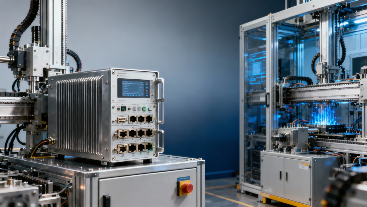
MTBF, or Mean Time Between Failures, is a statistical estimate of expected operating time between inherent failures for repairable equipment. It is not a service life guarantee, not a warranty term, and not proof that a box PC or fanless controller will run failure-free for 8 to 10 years. In many industrial settings, that misunderstanding starts at the specification sheet.

One common problem is that industrial pc MTBF calculation methods are based on component reliability handbooks rather than full-system stress exposure. That approach can be useful for baseline design review, but it can also omit installation variables such as 45°C cabinet heat, dust loading, 3-axis vibration, or daily power cycling. A system rated for indoor lab assumptions may behave very differently on a CNC line, AGV charging station, or roadside edge cabinet.

Another issue is the difference between predicted reliability and observed field reliability. A vendor may calculate MTBF from individual parts under nominal temperatures, while the buyer expects the figure to reflect installed operating reality. If a system uses 12 to 18 key subsystems—CPU board, SSD, power input, connectors, RAM, I/O modules, and thermal interfaces—small assumption errors can compound.

This matters because financial risk scales quickly. In a 100-unit edge deployment running 8,760 hours per year, even a modest reliability overstatement can alter expected failure events across a 3-year planning horizon. That affects maintenance staffing, replacement inventory, and service-level commitments to production or logistics operations.

Predicted MTBF is not the same as field failure behavior

Predicted MTBF is typically derived from accepted methods such as parts count or parts stress analysis. These methods are useful for design benchmarking, but they are sensitive to temperature, duty cycle, and environmental assumptions. If a supplier uses 25°C ambient while your enclosure regularly reaches 40°C to 55°C, the published number can become directionally misleading.

Field failure behavior, by contrast, reflects interactions between electronics, housing design, mounting orientation, vibration transfer, power quality, and workload peaks. For industrial buyers, the practical question should be: under what exact conditions was the industrial pc MTBF calculation made, and how closely do those conditions match deployment reality?

Core interpretation checkpoints

• Was the value modeled at 25°C, 40°C, or another ambient temperature range?
• Did the calculation include storage devices, connectors, power modules, and thermal interfaces?
• Was the workload assumed to be steady, bursty, or near 80% CPU utilization?
• Does the stated MTBF represent a complete system, a motherboard only, or a critical subassembly?

The calculation mistakes that most often skew risk

The biggest errors in industrial pc MTBF calculation are rarely mathematical mistakes alone. They are scope and assumption mistakes. A reliability figure can look precise to the hour while still failing to represent what matters operationally. That is why engineering review should focus on what was counted, what was ignored, and what stress model was used.

The table below outlines frequent sources of distortion seen in industrial procurement and technical comparison. These are especially relevant for fanless industrial PCs, edge gateways, machine vision controllers, and embedded systems used in 24/7 automation lines.

The key takeaway is that a single published value can be technically valid inside a narrow model and still be commercially misleading for real installations. Buyers should ask for the operating assumptions, included components, and applicable reliability standard before accepting a figure as decision-grade data.

Four recurring blind spots in supplier comparisons

First, thermal simplification is widespread. Fanless industrial PC platforms depend heavily on chassis conduction, mounting orientation, and ambient airflow. If thermal resistance rises even modestly, semiconductor junction temperatures can increase enough to materially reduce expected reliability. A fanless pc thermal dissipation test is therefore not a marketing accessory; it is a central input to realistic MTBF interpretation.

Second, connector and power path reliability is frequently underweighted. In edge cabinets, mobile equipment, and factory cells with intermittent shock, connectors, DC input stages, and storage interfaces may dominate field returns. A motherboard-centered industrial pc MTBF calculation can miss these failure drivers.

Third, many calculations assume stable power and limited transients. Yet in actual deployment, brownouts, ripple, surge exposure, and switching noise can create hidden stress. If your site has repeated daily on/off cycles or unstable utility conditions, ask whether the MTBF estimate includes that electrical reality.

Fourth, vendors may compare systems across different standards or handbooks without making methodology differences obvious. A 70,000-hour result under one method cannot be treated as directly equal to 90,000 hours under a different component library, confidence model, or environmental class.

What engineers should verify before approval

1. Confirm whether the value is predicted, tested, or field-observed.
2. Request ambient temperature, workload, and duty-cycle assumptions in writing.
3. Check whether SSD endurance, power input stages, and I/O modules were included.
4. Compare reliability claims alongside thermal, vibration, and ingress protection evidence.

How thermal, workload, and environment reshape MTBF in real deployments

A reliable industrial PC in a climate-controlled control room may not remain equally reliable inside a sealed automation cabinet, on a machine frame, or in a roadside enclosure. Real deployment conditions alter component stress levels, and stress levels alter failure probability. This is where industrial pc MTBF calculation becomes either useful engineering or false reassurance.

Temperature is usually the first multiplier. For many electronics, a sustained increase of 10°C in a stressed region can significantly accelerate wear-out mechanisms, although the exact effect depends on materials and component class. That is why a published MTBF at 25°C should never be read as deployment-neutral. In fanless designs, internal hotspots around CPUs, NVMe or SATA SSDs, and VRM sections deserve attention.

Workload is the second multiplier. A system running light HMI visualization at 20% average load has a different thermal and electrical profile than one handling machine vision inference, local data logging, or predictive maintenance software. If CPU utilization moves from 25% to 75%, heat density and storage writes may rise enough to change expected field reliability.

The third multiplier is environment: vibration, airborne contaminants, humidity swings, and power quality. In CNC workshops, fine particulates and coolant-adjacent conditions may challenge seals, connectors, and thermal surfaces. In transport or mobile robotics, repeated shock and oscillation add mechanical fatigue to the equation. These factors rarely show up in a headline MTBF number.

Deployment variables that should be mapped before procurement

Before approving a platform, procurement and engineering teams should document the actual operating profile. That means cabinet or site temperature range, hours per day, power cycle frequency, average and peak CPU load, storage write intensity, and vibration exposure. Even 5 variables captured over a 2- to 4-week observation window can improve comparison quality dramatically.

The following table can be used as a practical screening framework when reviewing industrial PC suppliers for edge AI, machine control, data acquisition, or unmanned remote systems.

This kind of operational mapping helps separate acceptable approximation from dangerous oversimplification. It also gives buyers a more defensible basis for supplier negotiation, especially when comparing a lower-cost system with a premium fanless design claiming superior thermal stability.

A practical review sequence

• Start with the deployment temperature and enclosure condition, not the brochure number.
• Review fanless pc thermal dissipation test evidence under near-real loads.
• Check SSD type, write endurance class, and expected logging profile.
• Ask for reliability interpretation tied to your 3-year or 5-year lifecycle plan.

A better framework for buyers, operators, and decision-makers

Instead of treating industrial pc MTBF calculation as a single-pass filter, leading teams use a layered decision model. The first layer is baseline reliability prediction. The second is environmental fit. The third is serviceability, including parts availability, replacement time, and remote diagnostics support. The fourth is lifecycle economics over 36 to 60 months.

For operators, the issue is uptime. For procurement, it is total landed risk. For senior management, it is whether the deployed platform supports business continuity without hidden maintenance escalation. In all three cases, the best decision rarely comes from the highest MTBF headline alone. It comes from the best alignment between predicted reliability and application stress.

TSV’s data-first position is especially relevant here: parameters only become decision-grade when their measurement context is transparent. An honest reliability discussion should include thermal design evidence, workload assumptions, support response expectations, and realistic field replacement workflows. In many industrial settings, a system with a lower stated MTBF but better thermal validation and faster service response may represent lower operational risk.

For purchasing teams, this means building evaluation criteria that connect engineering data to commercial outcomes. For example, if a 4-hour line stoppage costs more than a 10% hardware price difference, then spare strategy, onsite replacement simplicity, and remote health visibility may deserve greater weight than a brochure-level MTBF gap.

Suggested procurement checklist for industrial PC reliability review

The checklist below is useful for mixed audiences, from technical evaluators to sourcing managers. It helps convert industrial pc MTBF calculation into a risk-managed buying decision rather than a paper comparison exercise.

This framework prevents teams from overpaying for a number that lacks context or underbuying a platform that appears cheaper but carries higher downtime exposure. It also creates a better audit trail for internal approval, vendor qualification, and cross-functional signoff.

Questions worth asking in supplier meetings

• What exact environmental assumptions were used in the industrial pc MTBF calculation?
• Can you share thermal test results at 40°C ambient and near-peak workload?
• Which failure-prone parts are field replaceable within 30 to 60 minutes?
• How does your support model reduce downtime risk over a 3-year to 5-year deployment?

FAQ: practical questions about MTBF and industrial risk

How should buyers compare two industrial PCs with different MTBF numbers?

Do not compare the numbers in isolation. First confirm whether both values were calculated using the same standard and similar assumptions. Then review temperature range, included components, and workload basis. A system quoted at 90,000 hours under light conditions may present higher real-world risk than one rated at 70,000 hours with better thermal validation and stronger service support.

Is a higher MTBF always better for CNC, edge AI, or machine vision applications?

Not necessarily. In data-heavy applications, SSD endurance, write behavior, and cooling effectiveness may matter more than a headline MTBF increase of 15% to 20%. For CNC and machine vision workloads, buyers should also evaluate thermal saturation, I/O stability, and replacement simplicity under production schedules.

What is the most overlooked reliability input in fanless systems?

Thermal path integrity is often the most overlooked factor. If chassis conduction, mounting surface quality, or enclosure airflow differ from test conditions, internal temperatures can rise quickly. That is why fanless pc thermal dissipation test data should be reviewed together with installation orientation and cabinet layout, especially above 40°C ambient.

How often should reliability assumptions be revisited after deployment?

For new rollouts, a review after the first 3 to 6 months is sensible, followed by annual reassessment. If the deployment is in harsh conditions, includes 24/7 workloads, or supports high-cost production lines, quarterly trend checks on temperature, storage health, and event logs can help align maintenance planning with actual stress behavior.

Industrial PC reliability should be treated as an engineering context problem, not a brochure headline problem. When industrial pc MTBF calculation assumptions are hidden, incomplete, or detached from deployment conditions, risk gets skewed across budgeting, supplier selection, maintenance planning, and operational continuity. The most resilient buying decisions come from combining MTBF review with thermal evidence, workload mapping, environmental fit, and service readiness.

For teams evaluating industrial computing platforms in automation, CNC, edge AI, robotics, or remote infrastructure, TSV’s data-driven approach helps turn vague claims into measurable decision criteria. If you need a structured framework for supplier benchmarking, reliability review, or deployment risk analysis, contact us to discuss your application, request a tailored evaluation checklist, or explore more hard-tech decision support solutions.