Why EtherCAT cycle benchmarks differ from machine reality

EtherCAT cycle time benchmark figures often look impressive in lab reports, yet they rarely match what engineers see on running machines. Once cnc controller interpolation cycle, opc ua server response time, edge ai inference latency industrial loads, and real-time control contention enter the picture, deterministic timing shifts fast. This article explains why test-bench numbers diverge from production reality and how teams can evaluate motion, network, and control performance with engineering-grade rigor.

For R&D teams, machine builders, operators, procurement managers, and executive decision-makers, the gap is not academic. A published 250 µs EtherCAT cycle can become a 500 µs to 1 ms practical control window once servo drives, PLC tasks, HMI requests, safety traffic, and analytics workloads compete for the same compute budget. That difference affects contour accuracy, spindle synchronization, reject rate, and commissioning time.

At TechStat Vanguard, the useful question is not whether a benchmark number is technically possible. The useful question is whether that number survives under production constraints: multi-axis interpolation, OPC UA polling, edge AI inspection, thermal drift, logging, and maintenance diagnostics. Engineering truth starts where isolated lab performance ends.

Why lab-grade EtherCAT cycle benchmarks rarely survive the shop floor

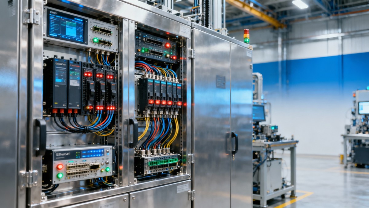
A cycle benchmark is usually measured under tightly controlled conditions: a limited node count, short cable runs, minimal background traffic, stable ambient temperature, and a lightly loaded CPU. In that environment, a controller may show 125 µs, 250 µs, or 500 µs cyclic exchange with low jitter. Those numbers are valid for the test setup, but they are not the same as machine reality.

On a production machine, the control stack becomes layered. The EtherCAT master exchanges process data, the cnc controller interpolation cycle computes trajectories, the motion kernel schedules servo updates, and the HMI triggers status reads. Add opc ua server response time for MES or SCADA integration, and the system no longer behaves like a single-purpose benchmark rig.

The biggest misunderstanding is to treat network cycle time as equal to application response time. A 250 µs bus cycle does not mean the machine reacts to a command in 250 µs. End-to-end latency often includes 4 to 8 stages: application task scheduling, fieldbus transfer, drive processing, actuator response, feedback acquisition, and supervisory confirmation. Each stage adds jitter and queueing risk.

In advanced manufacturing, even a small mismatch matters. A contouring machine cutting at 15 m/min with a 1 ms effective control update behaves differently from one maintaining stable control at 250 µs. The first may still meet general machining needs, but on high-dynamic corners, thin-wall parts, or synchronized gantry motion, path deviation, settling delay, and vibration become visible.

What benchmark reports usually omit

Many benchmark sheets do not state whether the controller was also running vision, data logging, recipe management, or external communications. They may publish average cycle time but omit jitter percentiles, such as 99th percentile or worst-case spikes over a 10-minute to 8-hour window. For machine builders, those omitted values often matter more than the headline minimum.

• Node count may be only 4 to 8 devices in the lab, while real machines can reach 20 to 80 nodes.
• CPU utilization may stay below 30% during tests, but integrated machines often run at 60% to 85% under peak events.
• Background traffic may be disabled during tests, while real systems exchange diagnostics, alarms, historian data, and remote access traffic.
• Benchmark windows may last 60 seconds, while production stability must hold for 8, 16, or 24 hours.

This is why procurement teams should never compare EtherCAT claims in isolation. The bus timing must be assessed together with controller architecture, task scheduling, communication stack design, and the intended machine duty cycle.

The four hidden latency contributors that reshape deterministic timing

When benchmark numbers diverge from field results, the root cause usually sits outside the fieldbus headline itself. In machine reality, four contributors dominate: cnc controller interpolation cycle length, opc ua server response time, edge ai inference latency industrial loads, and real-time control contention between tasks. Together, they define whether the machine feels crisp, acceptable, or unstable.

The cnc controller interpolation cycle is often the first limiting factor. Even if EtherCAT exchanges data every 250 µs, interpolation may run at 500 µs, 1 ms, or 2 ms depending on axis count, look-ahead depth, and contouring complexity. If the interpolation task is slower than the bus, the machine cannot exploit the nominal network speed.

The opc ua server response time becomes relevant once production data flows upward. An OPC UA service thread that handles subscriptions, historical reads, and external client requests can consume CPU and memory bandwidth. On integrated platforms, bursts of 50 to 200 tag updates per second can influence scheduling enough to increase motion jitter if task priorities are not isolated properly.

Edge AI inspection adds another layer. A vision model that infers in 8 ms on an unloaded edge device may stretch to 18 ms or 25 ms when image pre-processing, disk writes, timestamp alignment, and GPU/CPU sharing occur simultaneously. That is manageable if decoupled from real-time control, but risky if developers let non-real-time workloads compete on the same compute path.

How each contributor changes the real control envelope

The following table separates these timing domains. This matters because many teams try to fix a machine issue by focusing on EtherCAT alone, when the bottleneck sits one layer higher.

The practical conclusion is straightforward: deterministic timing is a stack property, not a single-benchmark property. A strong EtherCAT number is useful only when interpolation, analytics, and supervisory traffic are designed to coexist without priority inversion or compute starvation.

Real-time control contention is usually the final trigger

Contention appears when tasks with different deadlines compete for CPU cores, memory bandwidth, interrupt service time, or shared buses. For example, a motion loop needing sub-1 ms regularity can be disrupted by logging spikes, camera DMA transfers, or a software update service. The issue is not that any single task is too large. The issue is that timing-critical and non-timing-critical tasks were not partitioned correctly.

How to evaluate EtherCAT performance with engineering-grade rigor

A credible evaluation method starts by separating three measurements: bus cycle time, control loop update time, and end-to-end machine response. Teams that mix them together often buy the wrong controller, overspecify the network, or blame a fieldbus for an application-layer problem.

For most industrial equipment, a useful test window should run at least 4 hours, and 8 to 24 hours is better when thermal effects and background services matter. Short 5-minute captures can miss sporadic jitter spikes caused by file rotation, status polling, or network management events. Worst-case behavior matters more than headline average in safety-critical or precision applications.

The test environment should mirror the real machine as closely as possible: full node count, target cable lengths, expected HMI activity, OPC UA subscriptions, data logging, and any edge AI workloads that will ship with the system. If the machine is expected to run 12 axes, 2 spindles, and 1 vision station, the benchmark should include them. Otherwise, the result is only a partial indicator.

Procurement teams should also ask for jitter distribution, not just nominal cycle. A platform that delivers 500 µs with ±20 µs jitter may outperform one advertising 250 µs with occasional 800 µs outliers. In machine tools, packaging, robotics, and inspection cells, outliers often drive quality loss and troubleshooting cost more than the average number does.

A practical 5-step validation workflow

1. Define the real machine load: axis count, I/O count, safety devices, HMI actions, OPC UA clients, and any AI or vision task frequencies.
2. Measure bus cycle and jitter over at least 4 hours under nominal and peak operating states, including start-up and recipe change events.
3. Measure cnc controller interpolation cycle consistency under simple motion and high-curvature, multi-axis trajectories.
4. Stress supervisory traffic by simulating 50, 100, or 200 tag subscriptions and logging bursts to observe opc ua server response time impact.
5. Correlate timing with machine quality metrics such as path error, reject rate, settle time, or scan completion time.

This workflow links timing to operational outcomes. That matters because a procurement decision should not be based only on microseconds. It should be based on whether the platform meets tolerance, throughput, maintainability, and integration requirements without excessive engineering overhead.

Recommended metrics to request from vendors

The table below helps buyers and technical evaluators ask better questions during supplier review. It is designed for mixed audiences: machine builders, end users, and decision-makers comparing integrated automation platforms.

A supplier that can answer these questions clearly is usually more mature than one offering only a headline EtherCAT cycle figure. For serious capital equipment, transparency in timing architecture is often a stronger signal than marketing language about performance leadership.

Selection criteria for machine builders, operators, and procurement teams

Different stakeholders care about different timing outcomes. Operators want stable machine behavior and fewer nuisance faults. Engineers want repeatable interpolation and maintainable architecture. Procurement wants lower integration risk and shorter qualification cycles. Executives want throughput, uptime, and a clear return on automation investment. A realistic selection process has to convert timing metrics into business impact.

For machine builders, the first check is architectural fit. If the design requires 16 to 64 axes, synchronized camming, or high-speed contouring, then controller compute capacity, scheduling model, and drive feedback architecture matter as much as EtherCAT speed. For a simpler conveyor or pick-and-place cell, a 1 ms loop may be fully adequate, and chasing 250 µs may add cost without measurable production gain.

For procurement teams, the hidden cost lies in integration and support. A platform that benchmarks well but requires 6 to 12 extra engineering weeks for OPC UA tuning, AI workload isolation, or jitter troubleshooting may be less attractive than a slightly slower but more stable platform. Total deployment risk should be part of the bid comparison, not an afterthought after purchase order approval.

For plant decision-makers, uptime and traceability often outweigh absolute minimum cycle numbers. If a system can sustain production for 3 shifts with bounded jitter, clear diagnostics, and predictable serviceability, that may deliver more value than a theoretically faster controller that becomes fragile under mixed workloads.

A practical decision checklist

• Map timing needs by application class: packaging, CNC, robotics, inspection, or hybrid cells all have different acceptable latency envelopes.
• Request production-like benchmark conditions, including full node count and external communication loads.
• Verify whether edge AI inference latency industrial workloads run on isolated compute resources or share the same real-time controller.
• Confirm recovery behavior after alarms, warm restarts, and network reconnection events, not only steady-state performance.
• Compare 3 cost layers: hardware price, integration hours, and troubleshooting exposure over the first 12 months.

Typical fit by application complexity

A useful rule of thumb is this: if your process tolerance is forgiving and motion is discrete, a stable 1 ms architecture can be enough. If your process depends on synchronized contouring, high-speed metrology, or tightly coupled actuation and inspection, the review must go deeper into interpolation stability, jitter envelopes, and task isolation policies.

Common mistakes, risk controls, and FAQ for real-world benchmarking

The most common mistake is treating one benchmark screenshot as procurement evidence. A single lab capture cannot substitute for a structured validation plan. Another mistake is optimizing one layer while ignoring the others, such as reducing EtherCAT cycle time from 500 µs to 250 µs while leaving OPC UA traffic and AI inference on unmanaged shared resources.

A second risk is underestimating scaling effects. Machines often start with 8 axes and end with 12, or they begin with local HMI only and later add MES, historian, and remote diagnostics. What looked stable at 40% compute load can become unstable at 75% when new functions are activated. Procurement specifications should account for a 20% to 30% expansion margin where possible.

A third mistake is failing to define acceptance criteria. Teams should set thresholds before testing. For example: maximum control jitter under peak load, minimum acceptable opc ua server response time for a given tag rate, maximum inference delay for edge inspection, and allowable restart-to-ready time after a controlled interruption. Without predefined thresholds, benchmark discussions become subjective.

The right risk control approach is simple: test as shipped, measure over meaningful duration, isolate timing domains, and judge performance against process quality. That framework aligns engineers, operators, and buyers around the same operational truth.

FAQ: What buyers and engineers ask most often

Does a faster EtherCAT cycle always improve machine performance?

No. If the cnc controller interpolation cycle stays at 1 ms, or if task contention adds large jitter, a 250 µs bus may provide limited real benefit. The gain depends on whether the rest of the control stack can use that faster exchange deterministically.

What is a reasonable benchmark duration for supplier comparison?

For preliminary screening, 1 to 4 hours can reveal obvious instability. For production qualification, 8 to 24 hours is more credible, especially when thermal change, logging rotation, and network supervision can trigger intermittent latency spikes.

How should OPC UA be considered during control evaluation?

Treat opc ua server response time as part of system architecture, not an optional add-on. If the machine will expose 100 tags per second to MES or SCADA, that load should be present in testing. Otherwise, the validation misses a known production burden.

Can edge AI and real-time motion coexist on one platform?

Yes, but only with clear partitioning. Separate cores, bounded resource access, prioritized task scheduling, and careful buffering are usually required. Without those controls, edge ai inference latency industrial workloads can destabilize deterministic control even when average CPU load looks acceptable.

EtherCAT cycle benchmarks are useful, but only when interpreted in the full context of interpolation, supervisory traffic, AI workload, and task contention. For advanced manufacturing, the winning platform is not the one with the most dramatic lab number. It is the one that holds timing discipline under real machine conditions, supports maintainable integration, and protects process quality over long production windows.

If your team is comparing controllers, motion platforms, or integrated automation architectures, TechStat Vanguard can help you turn benchmark claims into engineering-grade evaluation criteria. Contact us to discuss a data-driven validation framework, request a tailored comparison methodology, or explore broader hard-tech benchmarking support for motion, network, and control systems.