Industrial robots energy efficiency comparison: where savings are real

For enterprise decision-makers, an industrial robots energy efficiency comparison is only useful when it goes beyond marketing claims and examines measurable power draw, duty cycles, payload matching, and real operating conditions. This introduction frames where energy savings are genuinely achievable, helping manufacturers reduce total cost of ownership while making data-driven automation investments grounded in engineering reality.

In practice, the largest savings rarely come from a single “low-power robot” label. They come from system-level engineering: selecting the right payload band, reducing idle time, tuning acceleration profiles, matching end-of-arm tooling mass, and measuring energy use per completed cycle rather than nameplate consumption alone. For CTOs, plant leaders, and procurement teams, the goal is not to buy the robot with the lowest brochure wattage, but to identify where 8%–25% energy reduction is actually feasible across a line, cell, or multi-site deployment.

That is where a rigorous industrial robots energy efficiency comparison becomes commercially useful. It helps separate fixed base consumption from motion-related demand, clarifies how collaborative robots differ from higher-payload articulated units, and reveals why a robot that appears efficient in a lab may underperform in 24/7 industrial duty. For organizations aligning automation strategy with measurable operating cost control, energy efficiency must be evaluated as an engineering variable, not a marketing promise.

What an Industrial Robots Energy Efficiency Comparison Should Actually Measure

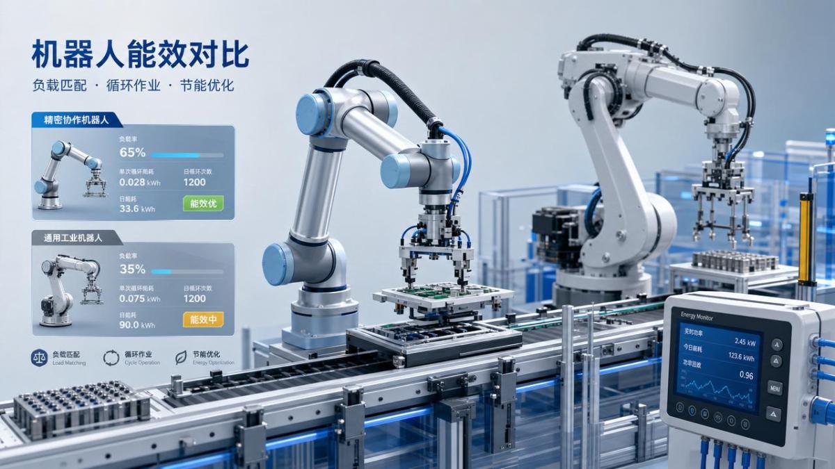
A credible industrial robots energy efficiency comparison starts with four measurable layers: baseline idle power, average cycle power, peak transient demand, and energy consumed per productive unit. Many buying teams only review installed motor ratings in kW, but that figure alone says little about real annual electricity cost. A 6-axis robot rated for a 20 kg payload may draw modest average power in a pick-and-place cell, while a lighter unit can consume more per good part if it is repeatedly overloaded, poorly programmed, or paired with heavy tooling.

The Four Core Measurement Dimensions

To compare robots in a procurement context, decision-makers should require at least 4 comparable metrics captured over the same test window, typically 30 minutes, 2 hours, and one representative shift. This creates enough data to distinguish startup spikes from steady-state operation.

• Idle or standby consumption during waiting states
• Average power during standard production cycles
• Peak draw during acceleration, braking, or rapid repositioning
• kWh per completed cycle, part, pallet, or weld seam

This matters because robots do not consume energy in a linear way. In many cells, 20%–40% of available shift time is non-productive waiting, indexing, or safety hold. If standby power is high, annual waste can become material even when the robot is mechanically efficient during movement.

Why Nameplate Ratings Mislead Buyers

Nameplate motor ratings reflect design capacity, not normal electricity use. A robot with multiple servo axes may be specified for high instantaneous output but operate most of the day at a fraction of that level. Procurement teams that compare only rated power often misjudge total cost of ownership by 10% or more, especially when auxiliary equipment such as grippers, vacuum pumps, vision lighting, and safety controllers are excluded from the model.

The table below outlines how different measurement points affect an industrial robots energy efficiency comparison in real purchasing decisions.

The key conclusion is simple: energy efficiency only becomes decision-grade when consumption is normalized against output. For high-mix, medium-volume manufacturers, this prevents false savings assumptions and supports more accurate ROI modeling over 3–7 years.

Where Energy Savings Are Real in Robotic Cells

Across most industrial environments, real savings do not come equally from every design choice. The strongest gains usually appear in 5 areas: payload right-sizing, motion optimization, reduced idle states, lighter tooling, and integrated peripheral control. In mature automation programs, these levers often outperform headline efficiency claims from robot hardware alone.

1. Payload Matching Prevents Structural Overbuying

One of the most common oversights is choosing a robot with 30%–60% more payload capacity than the application requires. While this may look like future-proofing, oversized robots often carry larger motors, heavier arms, and higher inertia. If a process needs to move 7 kg including gripper and cable dress, specifying a 20 kg robot can increase energy use without improving throughput.

A disciplined industrial robots energy efficiency comparison should therefore include total moving mass, not payload alone. That means product weight, end-effector, vacuum lines, sensor mounts, and any additional brackets. In many packaging, electronics, and light assembly cells, trimming tooling mass by 1 kg–3 kg can noticeably reduce repeated acceleration demand.

2. Motion Profiles Usually Matter More Than Maximum Speed

Plants often assume that faster robots are inherently more efficient because cycle time drops. The reality is more nuanced. Aggressive acceleration, abrupt stops, and unnecessary path complexity can raise peak draw and mechanical wear. In some applications, a 5% longer cycle with smoother trajectory planning reduces electricity use per part while maintaining line balance.

This is especially relevant in welding, palletizing, adhesive dispensing, and machine tending, where repeated path consistency matters more than burst speed. Programming teams should evaluate not just seconds per cycle, but energy per accepted output over a full production window of 8–12 hours.

3. Idle Time Is a Hidden Cost Center

A robot that waits for upstream conveyors, part presentation, manual loading, or vision confirmation can consume power without creating output. In some mixed-manufacturing cells, idle and blocked states account for 15%–35% of scheduled time. Energy savings become real when robot sleep logic, staged servo enable, and coordinated cell controls reduce unnecessary energized waiting.

The following comparison shows where savings typically come from and how significant they can be under common industrial conditions.

The practical takeaway is that savings are cumulative. A plant may only gain 4% from a better robot choice alone, but 12%–20% when hardware selection, programming, and auxiliary load control are optimized together.

How Robot Type Changes the Energy Equation

Not all robot classes should be compared in the same way. Collaborative robots, standard 6-axis articulated robots, SCARA platforms, and delta robots serve different motion envelopes and payload bands. An industrial robots energy efficiency comparison must be architecture-aware, otherwise the conclusions become misleading.

Collaborative Robots

Cobots often present favorable power profiles in light-duty applications because payloads may range from 3 kg to 16 kg and speeds are intentionally limited for shared environments. They can be energy-effective in electronics, inspection, or flexible assembly, especially where redeployment matters. However, if a line requires high throughput, a cobot may consume more energy per part simply because cycle time is longer.

Articulated Industrial Robots

These remain the workhorse for welding, palletizing, machine tending, and heavy handling. Their absolute power draw is usually higher, but energy per output can still be lower when throughput is significantly greater. For 20 kg, 60 kg, or 120 kg classes, the correct comparison metric is rarely instantaneous power; it is productive energy normalized over output volume and uptime.

SCARA and Delta Robots

For high-speed horizontal assembly or lightweight packaging tasks, SCARA and delta robots can deliver excellent efficiency because their kinematics are optimized for short, repetitive motions. In plants running thousands of cycles per shift, even a 0.02 kWh reduction per 100 cycles scales into meaningful annual savings. But these gains disappear if the application requires orientation flexibility they were not designed for.

Selection Questions Decision-Makers Should Ask

1. What is the real moving mass, including tooling and cable package?
2. How many cycles per hour must the cell sustain at acceptable quality?
3. What percentage of shift time is active motion versus waiting?
4. Will the robot run 1 shift, 2 shifts, or 24/7?
5. Can peripheral devices be power-managed with the robot controller?

These 5 questions typically reveal more about energy economics than vendor claims about “advanced efficiency.” They also help procurement teams compare offers across different robot classes without oversimplifying the business case.

A Procurement Framework for Energy-Focused Automation Decisions

For enterprise buyers, the most useful industrial robots energy efficiency comparison is embedded in a broader sourcing framework. That framework should combine technical fit, electricity consumption, maintainability, and implementation risk. A low-energy robot that requires frequent reprogramming, constrained spare parts access, or unstable cycle performance can lose its financial advantage within 12–24 months.

Build the Evaluation Around Total Cost of Ownership

A practical TCO model should cover at least 6 cost blocks: acquisition, integration, energy, maintenance, downtime risk, and end-of-life flexibility. Energy usually represents a smaller share than labor or downtime, but it becomes strategic across large fleets, especially when plants face rising power tariffs or internal carbon reporting requirements.

Recommended Vendor Data Package

When requesting quotations, buyers should ask vendors or integrators for a documented energy profile under three conditions: idle, nominal production, and peak motion. A 30-day pilot is ideal, but where that is not practical, a validated simulation plus application-specific assumptions can still provide decision value.

• Measured or modeled kWh per hour at expected duty cycle
• Cycle time at target payload and reach
• Tooling mass assumptions and compressed air usage
• Standby logic and restart behavior after stops
• Maintenance interval assumptions over 12 months

Common Buyer Mistakes

The first mistake is evaluating the robot without the cell. The second is assuming all savings come from the arm itself. The third is ignoring utilization rate. A robot running at 35% real utilization will have very different efficiency economics from the same unit running at 80% utilization, even with identical hardware. That is why engineering-led sourcing should test operational assumptions before approval.

Implementation, Monitoring, and Continuous Savings Verification

Once the robot is installed, energy performance should not remain a one-time selection exercise. Plants that achieve sustained savings usually adopt a 3-stage process: baseline measurement, control optimization, and periodic verification. Without this loop, actual performance can drift as product mix changes, tooling is modified, or operators override programmed states.

Stage 1: Baseline the Cell

During the first 2–4 weeks after commissioning, record hourly consumption, cycle count, and stop reasons. This allows teams to calculate energy per productive unit and identify whether the biggest losses come from motion, waiting, air consumption, or peripheral devices.

Stage 2: Optimize Control Logic

Typical improvements include servo standby modes, coordinated peripheral shutdown, vision-trigger sequencing, and path refinement. In many cells, the first optimization round can deliver a measurable 5%–10% reduction without hardware replacement.

Stage 3: Revalidate Quarterly

Quarterly review is often sufficient for stable lines; monthly review may be justified in high-volume operations. The point is to confirm that savings persist under actual product changeovers, seasonal demand swings, and maintenance conditions. A robot that was efficient at launch can become less efficient if grippers gain mass, payloads increase, or cycle paths are modified without re-optimization.

What This Means for Enterprise Strategy

For multi-site manufacturers, standardizing energy measurement across robotic cells creates a more reliable capital allocation model. It also supports supplier comparison, retrofit prioritization, and internal benchmarking. Instead of asking which robot brand is “most efficient,” leadership can ask which application architecture delivers the lowest verified energy per unit of output.

A meaningful industrial robots energy efficiency comparison does not reward the most persuasive brochure. It rewards the best engineering fit between payload, cycle design, duty pattern, and cell control. Real savings are typically found in right-sized robot selection, lower idle losses, smoother motion, lighter tooling, and continuous verification after deployment.

For decision-makers who need fewer assumptions and better technical clarity, TSV’s data-first approach helps turn robotic energy evaluation into a practical sourcing framework. If you are assessing a new automation project, comparing suppliers, or refining the total cost of ownership for an existing robotic cell, contact us to discuss a tailored benchmarking approach, request a customized comparison model, or learn more solutions grounded in engineering data.