CNC controller interpolation cycle and surface finish

In precision machining, the CNC controller interpolation cycle directly shapes contour accuracy, feed stability, and final surface finish. For engineers, buyers, and plant leaders comparing predictive maintenance software for CNC or evaluating digital twin simulation accuracy, understanding this parameter is essential. This article explains how interpolation timing affects machining quality, process reliability, and data-driven optimization in modern manufacturing.

For TSV’s audience, this is not a theoretical control-system detail. The interpolation cycle influences whether a machine can maintain commanded feed on tight curves, whether a mold cavity shows visible faceting, and whether a supplier’s process capability is repeatable across shifts, materials, and production batches. In aerospace, medical, robotics, and high-mix industrial parts, those differences can affect rework rates, inspection burden, and supplier qualification time.

A shorter cycle is not automatically better in every case, and a smoother finish is not determined by spindle speed or cutter geometry alone. Servo tuning, look-ahead, block processing speed, CAM output density, and machine stiffness all interact. The practical question is how to interpret interpolation timing as part of a larger machining performance benchmark, especially when selecting equipment, validating digital models, or improving CNC maintenance strategy.

What the CNC controller interpolation cycle actually does

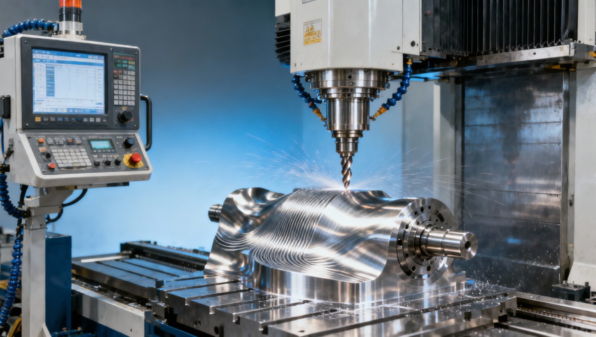
The interpolation cycle is the controller’s internal update interval for calculating the next commanded motion point along a programmed path. In simple terms, it determines how often the CNC recalculates axis positions, feed commands, and coordinated movement. Common interpolation cycle ranges in industrial CNC systems fall between 0.5 ms and 8 ms, depending on controller class, processing architecture, and machine application.

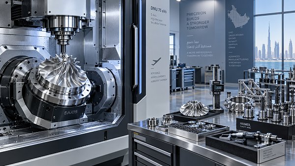
When the cycle is longer, the controller updates motion less frequently. On straight cuts at moderate feed rates, that may be acceptable. On complex 3D contours, small radii, impeller blades, thin-wall aerospace parts, or medical components with tight scallop limits, a long update interval can create chordal deviation, feed fluctuation, and visible waviness. That is why two machines with similar spindle power may produce very different surface quality on the same CAM program.

The cycle also matters for machine dynamics. At 10 m/min, a 1 ms interpolation cycle corresponds to a commanded travel step of about 0.167 mm, while a 4 ms cycle corresponds to about 0.667 mm before the next motion update. In practice, look-ahead and spline processing soften this effect, but the numerical relationship explains why high-speed contouring places more demand on fast control loops and strong servo coordination.

Interpolation is not the same as servo loop speed

A frequent mistake in procurement and specification review is to confuse interpolation cycle, position loop cycle, and current loop cycle. A controller may advertise a sub-millisecond servo loop, while the interpolation cycle that processes program path blocks is longer. For surface finish analysis, the distinction matters because path generation, axis command refresh, and drive response do not contribute equally to final part quality.

Operators and manufacturing engineers should therefore ask for at least 4 technical details during equipment comparison: interpolation cycle, look-ahead block capacity, supported spline or NURBS functions, and effective feed maintenance on small-radius contouring. Without those data points, “high-speed machining” claims remain too vague for serious sourcing decisions.

Why this matters in benchmarking

TSV’s engineering-centered approach treats interpolation timing as one benchmark variable among several measurable variables. A reliable benchmark should compare the same material, same tool diameter, same radial engagement, same tolerance target, and same CAM strategy. Otherwise, surface finish differences get incorrectly attributed to the controller alone.

The table below shows how interpolation timing typically interacts with contouring behavior in real machining environments.

The key takeaway is that interpolation cycle should be matched to the intended geometry and feed regime. For procurement teams, this means a shorter cycle creates the most value when the part mix includes high-curvature surfaces, tolerance bands below ±0.01 mm, or visible cosmetic finish requirements that drive downstream polishing cost.

How interpolation timing affects surface finish in real production

Surface finish is influenced by several layers of the machining system, but interpolation timing has a direct role in how smoothly the cutter tracks the intended path. If the commanded motion is updated too coarsely, the machine may decelerate repeatedly in short segments, especially when CAM output contains many small linear blocks. The result can be micro-stop marks, uneven tool loading, and a measurable rise in Ra or Rz values.

In finishing operations on aluminum, stainless steel, titanium, hardened steel, and engineering polymers, engineers often see the strongest impact at feed rates above 3 m/min to 15 m/min on dense 3D toolpaths. On a freeform cavity, one setup may hold Ra 0.4–0.8 µm with stable motion, while a less capable motion system on the same nominal program may drift to Ra 0.8–1.6 µm or require slower feed to recover finish quality.

This effect is not only cosmetic. Poor feed continuity can raise local heat input, worsen burr formation at edge transitions, and accelerate tool wear. A finish pass that should run in 12 minutes may take 16–18 minutes once the operator reduces feed override to suppress visible patterning. Over hundreds of parts per month, that difference becomes a capacity and cost issue, not merely a quality issue.

Three common surface finish failure patterns

• Facet-like texture on curved surfaces caused by coarse block execution relative to feed rate and geometry density.
• Witness marks at direction changes where feed drops too sharply and the cutter lingers momentarily.
• Periodic waviness linked to combined effects of interpolation timing, servo lag, and insufficient dynamic smoothing.

For process engineers, the practical challenge is separating controller behavior from tooling and machine mechanics. A surface defect that appears every 0.5 mm to 2 mm along a contour may suggest motion update or servo interaction. A more random finish problem may point to spindle vibration, tool imbalance, coolant issues, or material inconsistency. Good diagnostics require synchronized review of NC code type, feed trace, servo load trend, and actual finish measurements.

Why CAM strategy still matters

Even a fast controller can underperform if the CAM output overwhelms block processing. In many shops, switching from short-line approximation to spline-based output, or increasing tolerance intelligently from 0.001 mm to 0.005 mm in non-critical regions, reduces data load without harming part function. That can improve feed stability and shorten cycle time while keeping the required finish window intact.

For digital twin validation, this is critical. If the simulation assumes ideal continuous motion but the real machine is executing heavy segmented code with limited look-ahead, predicted finish and real finish may diverge. The interpolation cycle becomes a bridge parameter between virtual process planning and actual shop-floor behavior.

Key parameters engineers and buyers should evaluate together

Interpolation cycle should never be reviewed in isolation. In supplier comparison, machine acceptance, or controller retrofit assessment, the more useful question is how the full motion architecture performs as a system. A robust evaluation usually includes at least 6 technical dimensions: interpolation cycle, look-ahead depth, contour tolerance control, supported motion format, servo response quality, and actual finish performance on a reference part.

For procurement teams, this broader view reduces the risk of overpaying for specifications that do not translate into production value. A 1 ms interpolation cycle with weak tuning or poor CAM-controller matching may underperform a 2 ms system with superior smoothing and higher block-processing capability. Decision-makers should therefore request demonstration conditions, not only brochure values.

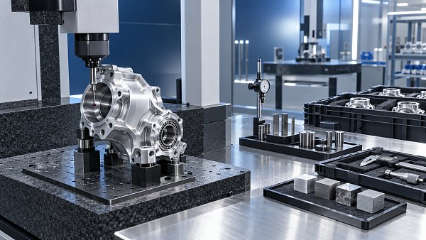
The most useful benchmark parts are geometry-rich and repeatable. Examples include a stepped-radius contour, a thin-wall pocket, a shallow 3D cavity, and a small-radius spiral toolpath. These test pieces reveal whether the machine can hold feed, whether corner transitions are clean, and whether the resulting surface requires secondary polishing.

A practical evaluation matrix

The table below can be used by engineering, operations, and sourcing teams during RFQ review or factory acceptance testing.

This matrix highlights a recurring point in hard-tech sourcing: parameters only matter when linked to measurable outcomes. Buyers should ask suppliers to document test conditions such as spindle speed, cutter diameter, stepover, workpiece material, and target tolerance. Without that context, surface finish comparisons are difficult to trust.

Recommended checks before purchase or retrofit

1. Run one standard 3D contour test at 2 feed settings, for example 4 m/min and 8 m/min.
2. Record actual feed trace, cycle time, spindle load, and final surface roughness.
3. Compare NC output in both segmented and smoothed formats if supported.
4. Review whether the same result can be repeated across at least 3 consecutive parts.

For senior decision-makers, these steps create a cleaner line between marketing claims and engineering truth. That is exactly where TSV’s data-first perspective is most valuable: it shortens the qualification loop and reduces the chance of selecting a machine on incomplete motion-control evidence.

How interpolation cycle connects to predictive maintenance and digital twins

Interpolation timing is usually discussed as a machining-quality topic, but it also matters in predictive maintenance and process simulation. If the control system is forced to process extremely dense toolpaths near its practical limit, axis acceleration demand, servo following error, and thermal load can increase. Over time, that may reveal weak points in drives, encoders, ballscrews, or guideways, especially on machines running two or three shifts.

Maintenance software that monitors feed override usage, following error trends, axis load peaks, and contour alarm frequency can identify whether finish problems stem from wear progression or from a poor match between program structure and controller capability. In many factories, the warning sign appears first as a gradual increase in manual feed reduction during finishing, often 5% to 20% over baseline, before any obvious alarm occurs.

For digital twins, interpolation cycle is a realism variable. A simulation that models cutter engagement but ignores motion update limitations can overestimate achievable feed stability and underestimate finishing time. This matters when planners use virtual models to quote lead time, estimate machine capacity, or compare one supplier site against another in a distributed manufacturing network.

Data points worth capturing

• Actual versus commanded feed during finishing passes on high-curvature geometry.
• Servo following error trends over 30, 60, and 90 days for the same part family.
• Surface roughness drift by machine, shift, tool life stage, and material batch.
• Alarm and override frequency when NC file size or block density increases above normal ranges.

When these signals are tied together, teams can decide whether to retune the servo system, alter the CAM output style, upgrade controller options, or schedule preventive service. This is a more disciplined response than simply lowering feed or adding polishing time, both of which hide root causes and erode margin.

Where plant leaders gain value

Plant managers and operations directors benefit because interpolation-aware monitoring supports better capacity planning. If one machine holds finish at 8 m/min while another needs 5 m/min for the same contour, the difference over a 20-hour weekly finishing load is substantial. It affects staffing, promised delivery dates, and total cost per qualified part.

For multinational sourcing teams, that same logic applies to supplier comparison. Shops that can show controlled interpolation-related performance, not just nominal machine brand names, are easier to qualify for demanding sectors such as aerospace structures, sensor housings, and precision automation components.

Selection guidance, implementation steps, and common mistakes

Whether you are buying a new machine, validating a contract manufacturer, or improving an existing cell, the right approach is to connect interpolation cycle to the specific business goal. A mold shop focused on mirror-ready finishing will prioritize different motion behavior than a job shop cutting mostly brackets and plates. The wrong specification can lead to overspending or underperformance.

A practical implementation plan usually has 3 stages. First, define the part families that matter most, including tolerance, surface finish target, and average feed regime. Second, run controlled comparison tests with a stable tool and material baseline. Third, decide whether the gap should be solved through CAM optimization, control options, maintenance, or machine replacement. This sequence prevents expensive changes based on assumptions alone.

Common mistakes to avoid

• Choosing by spindle speed or horsepower alone while ignoring contouring behavior on actual 3D programs.
• Assuming a fast interpolation cycle guarantees good finish even when tooling, fixturing, or machine rigidity are weak.
• Comparing supplier samples without matching material grade, cutter geometry, tolerance, and stepover conditions.
• Using digital simulation outputs that do not account for controller processing limits or feed smoothing behavior.

For procurement teams, it helps to define acceptance criteria before the trial. That can include a target roughness band such as Ra ≤ 0.8 µm, contour tolerance within ±0.01 mm, and a cycle-time ceiling within 10% of the quoted estimate. Clear criteria reduce subjective debate and make supplier evaluation more consistent across regions and departments.

FAQ: practical questions from engineers and buyers

How short should the interpolation cycle be for precision finishing? For high-value 3D finishing, many applications benefit from 0.5–2 ms, but the right number depends on feed rate, geometry complexity, and smoothing functions. A longer cycle can still perform well if the controller has strong look-ahead and optimized path handling.

Can interpolation issues be fixed without replacing the machine? Often yes. Shops may gain measurable improvement through CAM output refinement, servo tuning, software options, or maintenance on axes and feedback systems. The best starting point is a controlled before-and-after test on one representative part.

What should buyers request from suppliers? Ask for test-part conditions, actual feed trace, finish measurement method, and whether results were achieved with standard controller options or paid upgrades. This usually gives more decision value than a generic speed claim.

CNC controller interpolation cycle is a small parameter with large operational consequences. It influences contour accuracy, feed continuity, visible finish, maintenance insight, and the credibility of digital process models. For engineers, operators, sourcing teams, and executives, the most effective strategy is to evaluate it together with look-ahead, path format, servo behavior, and verified part results.

At TSV, the priority is always measurable engineering truth over marketing shorthand. If you are benchmarking machining capability, qualifying a precision supplier, or reviewing CNC optimization opportunities, a data-led assessment of interpolation cycle can reduce trial-and-error, clarify equipment value, and improve confidence in production decisions. Contact us to discuss a tailored evaluation framework, request a benchmarking checklist, or explore more precision machining analysis solutions.