How much does solid-state LiDAR cost in 2026?

In 2026, solid-state LiDAR pricing is no longer a simple hardware question—it reflects performance, integration cost, and deployment scale across AGV AMR, robotics, and edge sensing systems. For engineers, buyers, and decision-makers, understanding what drives solid-state LiDAR cost is essential to comparing specifications, avoiding marketing noise, and selecting data-backed solutions that fit real industrial requirements.

For most industrial teams, the real question is not whether a unit costs USD 120, USD 450, or more than USD 1,500. The practical question is what that price includes: sensing range, resolution, interference resistance, automotive or industrial qualification, software stack maturity, and long-term maintenance burden. A low quoted price can still produce a high project cost if integration takes 8 to 12 extra weeks or if false detections disrupt a warehouse fleet.

At TechStat Vanguard, the useful way to evaluate solid-state LiDAR cost is through engineering truth rather than advertising language. Buyers in robotics, UAV payload integration, machine perception, and smart infrastructure need cost visibility across the full decision chain: component selection, validation, interface compatibility, enclosure design, calibration, field commissioning, and lifecycle replacement planning.

What solid-state LiDAR typically costs in 2026

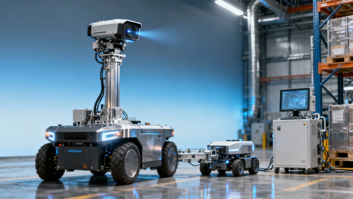
In 2026, solid-state LiDAR prices generally fall into several practical tiers rather than one market average. For short-range indoor navigation, entry-level units used in AGV or AMR platforms may sit in the USD 100 to USD 300 range in volume orders. Mid-range industrial sensors often land between USD 350 and USD 900, while higher-performance models for outdoor robotics, autonomous equipment, or demanding edge sensing can exceed USD 1,000 per unit.

These ranges vary based on order size, scan architecture, environmental protection level, and embedded processing features. A pilot purchase of 10 to 20 units can differ sharply from a 1,000-unit annual procurement agreement. In some projects, the same sensor family may show a 15% to 30% pricing gap depending on whether software development kits, synchronization accessories, or protective housings are bundled.

Another reason pricing appears inconsistent is that vendors often quote different cost boundaries. One quote may represent sensor-only hardware, while another includes firmware support, ROS drivers, calibration tools, or 12-month engineering support. Procurement teams that compare line items without standardizing the scope often misjudge the actual solid-state LiDAR cost by hundreds of dollars per deployment node.

The table below outlines common 2026 pricing bands by application logic rather than by marketing category. It is intended as a budgeting reference for technical screening and supplier qualification.

The key takeaway is that there is no single “correct” solid-state LiDAR price in 2026. Cost must be benchmarked against detection distance, angular resolution, frame rate, and deployment risk. A USD 250 sensor may be efficient for a 1.5 m/s indoor AMR, while a USD 1,400 unit may be justified for mixed-light outdoor navigation where false positives carry operational or safety consequences.

Why market averages can be misleading

Average pricing hides major differences in qualification grade, thermal range, and software support. A unit rated for 0°C to 40°C office conditions is not comparable to one validated for -20°C to 60°C industrial environments. Likewise, two sensors with similar range claims may differ materially in fog tolerance, retroreflector behavior, and cross-talk suppression when 20 or more robots operate in the same lane network.

The main cost drivers behind solid-state LiDAR pricing

The biggest mistake in sourcing is assuming that price mainly follows range. In reality, solid-state LiDAR cost is driven by at least five variables: optical architecture, receiver sensitivity, onboard compute, environmental durability, and software ecosystem maturity. Two sensors both rated at 100 m maximum range can have very different bill-of-material logic if one delivers usable perception only in controlled conditions and the other maintains stable output in rain, dust, or reflective industrial zones.

Resolution and point cloud structure also affect cost. Higher channel density or finer angular granularity improves object edge definition, docking accuracy, and path planning confidence. However, it also increases processing load. That means system cost may rise twice: once at the sensor level and again at the compute platform level if the host processor must move from a low-power edge module to a more capable industrial IPC or embedded GPU platform.

Reliability engineering adds another layer. Sensors intended for 24/7 duty cycles, vibration exposure, or IP65/IP67 installation require tighter packaging, stronger thermal design, and more stable internal calibration. This is especially important in logistics facilities, autonomous yard vehicles, or mobile robots that operate 16 to 20 hours per day. In such cases, replacement intervals and downtime cost can matter more than the purchase price itself.

The following table breaks down common factors that push cost up or down during evaluation and RFQ comparison.

A disciplined buyer should separate hardware cost from system cost. If a cheaper unit requires a custom synchronization board, external heaters, or 3 rounds of algorithm tuning, the total cost of ownership can rise by 20% to 50%. This is why engineering teams should ask for integration documentation, not just a datasheet excerpt.

H4-level evaluation logic for technical buyers

Ask what is validated under real operating conditions

A meaningful cost comparison should verify at least 4 items: target reflectivity assumptions, ambient light condition, test distance methodology, and packet output stability. Without these details, two quotes cannot be fairly compared, even if the listed field of view and nominal range look similar.

How application scenario changes the acceptable price point

Different industries tolerate very different price ceilings because the sensing task is different. In a low-speed indoor AMR with route speeds under 2 m/s, a short-range solid-state LiDAR may be sufficient when paired with bump sensors, safety controllers, and encoded wheel feedback. In contrast, an outdoor inspection robot or unmanned vehicle may need higher confidence at 50 m to 120 m, making a more expensive sensor operationally necessary.

For robotics and automation, pricing should be linked to navigation reliability, docking precision, and fleet density. A sensor that is 25% more expensive but reduces obstacle misclassification during peak traffic can protect throughput across dozens of vehicles. In logistics environments where one stalled AMR lane delays multiple stations, the indirect cost of poor perception often exceeds the sensor delta within 3 to 6 months.

In UAV and aerospace-adjacent testing, weight, power draw, and mounting complexity change the budget equation. A unit that saves 200 g and 5 W may allow longer endurance or smaller payload structures, which can justify a higher component price. The same principle applies to edge AI deployments in smart infrastructure, where the right LiDAR may reduce the need for multi-camera redundancy or heavy post-processing at the gateway level.

Instead of asking for the cheapest available quote, buying teams should define the application envelope first. The checklist below is a practical starting point for matching scenario to price tolerance.

• Operating speed: below 2 m/s, 2–5 m/s, or above 5 m/s.
• Required detection distance: 10–20 m indoor, 30–80 m semi-outdoor, or 100 m+ outdoor.
• Environmental stress: clean warehouse, dusty plant, rain exposure, vibration, or strong sunlight.
• Deployment scale: pilot of 5 units, site rollout of 50 units, or fleet program above 500 units annually.
• Compute architecture: local edge processing only, central fusion, or hybrid perception stack.

When these five factors are clearly defined, the acceptable solid-state LiDAR cost becomes much easier to defend internally. Procurement can then align CapEx with measurable engineering outcomes instead of generalized claims about “high performance.”

Typical industrial use-case mapping

A warehouse AMR, a curbside delivery robot, and a mapping UAV may all use solid-state LiDAR, but their price logic is not interchangeable. Each application values a different balance of frame rate, range, robustness, latency, and payload efficiency. That is why a good sourcing process starts with mission profile definition before vendor shortlisting.

How to compare quotes beyond sensor unit price

A quote comparison should include at least 6 cost layers: sensor hardware, mounting and enclosure, electrical interface, software integration, validation labor, and after-sales support. Many teams compare only the first layer and discover late-stage overruns when electromagnetic compatibility issues, firmware updates, or thermal packaging changes appear during field trials.

A disciplined RFQ should request specific information on data output format, synchronization options, ingress protection, mean replacement lead time, and recommended maintenance interval. If one supplier can ship within 2 to 4 weeks and another needs 10 to 14 weeks, that difference affects launch planning and safety stock strategy. The same applies to spare unit policy for fleets larger than 100 vehicles.

The table below provides a simple comparison framework that engineering, sourcing, and management teams can use together. It is designed to reduce ambiguity in cross-functional procurement reviews.

The practical conclusion is simple: the cheapest solid-state LiDAR quote is often not the lowest-cost option. In B2B deployment, integration friction, support latency, and field stability are measurable economic variables. A procurement team that standardizes these comparison items will usually make faster and safer decisions.

A 5-step sourcing process

1. Define mission profile and minimum sensing envelope.
2. Shortlist 3 to 5 suppliers with matching interface requirements.
3. Run bench validation for range, latency, and interference behavior.
4. Conduct field trial for at least 2 to 4 weeks.
5. Compare total deployment cost, not hardware alone.

Common buying mistakes, FAQs, and what decision-makers should do next

One common mistake is overbuying range and underbuying integration support. Another is selecting a sensor based on a perfect demo environment that does not represent the actual plant, yard, or mobile platform. A third mistake is ignoring replacement policy. In real deployments, mean service response time and spare availability can be more important than a small difference in list price.

Decision-makers should also distinguish between prototype economics and scale economics. A development team may accept a USD 1,200 evaluation sensor for fast testing, but a fleet business model can fail if the production sensor plus mounting and compute stack pushes the node cost beyond the allowable threshold. Many successful programs define a prototype budget, a pre-production budget, and a mass deployment target separately over 3 stages.

For data-driven organizations, the best approach is to align sourcing with measurable acceptance criteria: false positive tolerance, response latency, thermal envelope, service lead time, and integration man-hours. This creates an engineering-grade procurement process that cuts noise and lowers supplier qualification risk.

How much should an AGV or AMR project budget for solid-state LiDAR in 2026?

For many indoor AGV and AMR projects, a practical hardware budget may fall between USD 150 and USD 800 per sensing node, depending on speed, safety architecture, and redundancy strategy. Full deployed cost can be higher once brackets, wiring, compute upgrades, and validation effort are included.

Is lower-cost solid-state LiDAR always a risky choice?

No. Lower-cost sensors can be the correct choice when the environment is controlled, the required range is short, and the platform has secondary sensing layers. The risk begins when a low-cost unit is forced into harsh conditions or high-speed decision loops that exceed its validated operating envelope.

What should procurement ask suppliers before comparing price?

At minimum, request 6 items: validated range conditions, field of view, output interface, environmental rating, software tools included, and lead time for both production and replacement units. These details turn a marketing quote into an engineering quote.

Action point for engineering and sourcing teams

In 2026, solid-state LiDAR cost should be judged as a deployment variable, not a catalog number. Teams that benchmark price against usable performance, integration effort, and lifecycle support will make stronger decisions in robotics, automation, UAV, and edge AI programs. If you are building a supplier shortlist, refining a spec sheet, or validating an industrial sensing architecture, contact TechStat Vanguard to discuss a more data-backed comparison framework, request a tailored evaluation matrix, or explore solution guidance for your specific operating scenario.