Evaluate solid-state LiDAR point cloud density by measuring valid, spatially distributed returns on relevant targets at required ranges, within the time available for detection.
A high point count does not automatically establish reliable obstacle detection. Engineers need to know where measurements occur, which surfaces return signals, and how coverage changes.
Compare angular sampling, points per square meter, frame rate, and regional coverage under controlled reflectivity, lighting, and motion conditions before accepting a supplier’s headline specifications.
For engineering and procurement teams, the objective is straightforward: establish whether a sensor provides enough usable spatial detail to satisfy measurable application requirements consistently.
What Does Point Cloud Density Actually Tell You?
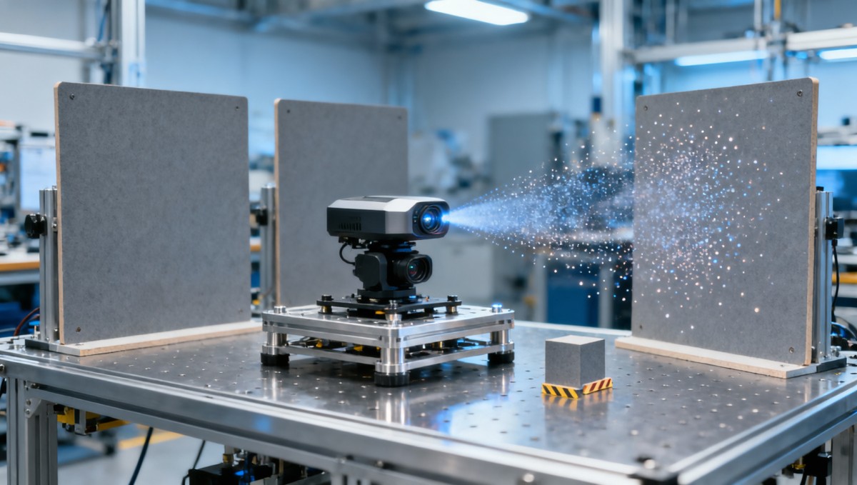
Point cloud density describes how closely measurements populate a defined spatial region during a specified interval. Its meaning depends on the denominator and counting rules.
Points per second measures output throughput. Points per frame describes a temporal grouping. Points per square meter describes sampling on a specified surface or projection.
None of these metrics alone establishes detection capability. A sensor can report many points while leaving a small, distant obstacle insufficiently sampled for reliable classification.
Start by separating emitted samples, reported returns, and accepted measurements. Missing returns, duplicate coordinates, and processing artifacts can make these quantities substantially different in practice.
A valid return should satisfy declared criteria for range, confidence, and plausibility. Those criteria must remain consistent across compared sensors, or differences become difficult to interpret.
Also distinguish sampling density from independent spatial resolution. Overlapping beam footprints or repeated measurements may increase point counts without resolving additional features on the target.
Which Density Metrics Should Engineers Compare?
A defensible comparison uses several complementary measurements. Each addresses a different failure mode, from inadequate angular spacing to concentrated coverage that conceals gaps elsewhere in view.
Ask suppliers whether their advertised rate counts multiple echoes from one emitted sample separately. Multiple returns can be valuable, but they do not add sampled directions.
Check whether reported density includes interpolation, upsampling, or accumulated frames. These outputs may support perception, but they require separate labeling from directly measured returns.
For procurement, request native measurement data alongside processed output when available. This helps reveal whether apparent coverage comes from sensor sampling or downstream reconstruction methods.
How Does Angular Sampling Translate Into Density at Range?
For a locally uniform angular grid, horizontal and vertical sample spacing increase approximately in proportion to range. Consequently, surface density decreases approximately with range squared.
For small angles, use sh ≈ RΔθh and sv ≈ RΔθv, with angular increments expressed in radians. These estimate spacing near a perpendicular target’s center.
The corresponding ideal surface density is approximately ρ ≈ 1/(R²ΔθhΔθv). This assumes distinct measurements, complete returns, and locally regular sampling on a perpendicular planar surface.
Consider an illustrative sensor with 0.2-degree spacing in both directions. At 20 meters, adjacent samples are approximately seven centimeters apart near the center of view.
That corresponds to roughly 205 samples per square meter under ideal conditions. At 40 meters, spacing doubles and theoretical density falls to approximately 51.
These values are geometric estimates, not measured performance claims. Dark surfaces, incidence angle, beam divergence, and missed returns can substantially reduce usable detail in practice.
Why Can Average Density Hide Critical Coverage Gaps?
Solid-state architectures can produce different spatial patterns. Flash, electronically steered, and scanning implementations should be compared through measured coverage rather than architecture labels alone.
Some suppliers also group MEMS-based scanning products under solid-state terminology. Confirm the steering mechanism and sampling behavior instead of assuming the label guarantees uniform coverage.
A sensor may concentrate measurements in a central region while sparsely sampling peripheral areas. Whole-frame averages can therefore exaggerate capability where your application needs coverage.
Divide the operational field of view into angular tiles and report valid measurements for each tile. Include center, edges, corners, and any configured priority region.
On a surveyed target surface, also calculate occupied-cell coverage: the proportion of predefined surface cells containing at least one accepted measurement during the evaluation interval.
Choose cell size from the smallest relevant feature, then report empty regions and largest gaps. A high average cannot compensate for an unsampled critical obstacle.
How Many Points Does Your Smallest Target Need?
Begin with the application’s minimum target size, required detection distance, and allowable response time. These requirements determine whether a given sampling pattern is sufficient.
For a perpendicular target under locally uniform sampling, expected samples are approximately its projected area multiplied by theoretical density. Actual valid returns require experimental confirmation.
Using the earlier example, a ten-centimeter square target at 20 meters corresponds to approximately two ideal samples. Alignment alone may change the observed count substantially.
Do not treat this average as a detection guarantee. Beam footprint, target boundaries, background mixing, and sampling alignment can produce fewer reliable returns than expected.
There is no universal minimum point count for detection. A simple obstacle alarm and a semantic classifier may require very different evidence from identical sensors.
Test the intended perception pipeline, including false alarms and missed detections. Density supports detection, while measured task performance determines whether the system meets its requirements.
How Should You Measure Points per Square Meter?
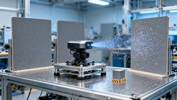
Use a planar target with surveyed dimensions and a documented orientation. Define its region independently of the observed point cloud to avoid selecting only successful returns.
For each frame, count accepted returns associated with that region and divide by its reference area. State whether the denominator represents actual or projected surface area.
For an inclined surface, the area presented to the sensor decreases with incidence angle. This changes surface sampling even before reflectivity and signal losses are considered.
Report raw valid-return density alongside occupied-cell coverage and repeated-hit statistics. Repeated measurements in one cell increase counts without improving coverage of neighboring empty cells.
Specify the distance tolerance used to associate points with the target plane. An excessively broad tolerance can admit background returns and inflate the density estimate.
Repeat measurements across many frames and target positions. Report distributions and worst-case gaps, because a single favorable frame can conceal unstable sampling or intermittent dropout.
Which Test Conditions Reveal Usable Density?
Build a test matrix around operating conditions that can reduce valid returns. At minimum, vary range, target reflectivity, incidence angle, ambient illumination, and sensor temperature.
Use targets with characterized reflectance near the sensor’s operating wavelength. Visible color alone does not reliably describe how strongly a material returns near-infrared light.
Document ambient conditions carefully. Lux describes visible illumination, so sunlight testing should also record geometry and, where practical, spectral irradiance relevant to the receiver.
Include wet, glossy, and dark surfaces when relevant to deployment. Such targets can produce dropouts, mixed returns, or geometry-dependent artifacts that bright boards conceal.
Introduce representative dust, rain, fog, or nearby LiDAR activity when the application requires them. Record unwanted returns and target retention separately from total point count.
Control mounting, power, warm-up, firmware, and operating mode throughout comparison. Otherwise, changes in exposure, filtering, or thermal behavior may be mistaken for inherent sensor differences.
Does Higher Density Come at the Cost of Response Time?
Point cloud density must be evaluated within the system’s decision window. Accumulating measurements for one second may look impressive while failing a rapid braking requirement.
Compare sensors using the same observation interval and region of interest. A supplier-defined frame may represent different scan durations or coverage cycles across products.
Measure acquisition duration, output latency, and the age of measurements entering the perception pipeline. Frame rate alone does not reveal when an obstacle becomes actionable.
For moving platforms, accumulated points require timestamping and motion compensation. Without them, dense clouds can smear edges, shift objects, and create misleading surface coverage.
Motion compensation also depends on calibration and pose accuracy. Report residual alignment error, since compensation can preserve apparent density while degrading the geometry needed for detection.
Benchmark at operational vehicle and target speeds. Confirm that coverage, processing time, and detection latency remain acceptable together, rather than optimizing point count in isolation.
What Evidence Should a Supplier Provide Before Selection?
Request a reproducible measurement package rather than a single density figure. It should identify hardware revision, firmware, operating mode, calibration, and all active processing settings.
Require the field of view, regional sampling pattern, frame definition, timestamp convention, and return-counting policy. Ask whether reported numbers are theoretical, typical, or guaranteed.
For range claims, request the target reflectance, target size, ambient conditions, and acceptance criteria. Maximum detection range does not establish adequate density at that distance.
Obtain representative recorded data and the method used to calculate density. Engineers should be able to reproduce the reported result from the supplied measurements.
Compare several units where qualification risk warrants it. Unit variation and thermal drift may matter more than a modest difference between advertised sampling rates.
Include integration costs in the decision: bandwidth, compute load, calibration effort, and maintenance. Additional points provide limited value if processing cannot meet the required deadline.
How Do You Turn Density Measurements Into a Selection Decision?
Define pass criteria before testing: required target detection rate, acceptable false alarms, maximum response time, and minimum coverage across the application’s operating envelope under evaluation.
Then use density measurements to explain successes and failures. Angular spacing reveals geometric limits, while regional coverage and valid-return rates expose gaps under realistic conditions.
A procurement comparison should connect each result to a requirement, including the test conditions and uncertainty. Avoid ranking sensors by one unqualified headline number alone.
The strongest solid-state LiDAR point cloud density benchmark establishes usable detail where and when it matters. Select the sensor that consistently satisfies the application’s measured requirements.