Interpreting Industrial IoT Latency Data for Monitoring and Real-Time Control

Interpreting Industrial IoT Latency Data for Monitoring and Real-Time Control

A low average latency can hide the timing failures that make an Industrial IoT system unsuitable for real-time control. Interpreting industrial category latency data requires more than comparing headline figures: measurement boundaries, clock synchronization, jitter, tail latency, and deadline misses all shape the result. A gateway that performs well in a telemetry demonstration may still be the wrong place to close a control loop.

The practical question is not simply “How fast is it?” It is “Will sufficiently fresh data reach the right application, and will the resulting action occur before its deadline under the conditions we actually expect?” That distinction should drive both technical evaluation and procurement specifications.

Monitoring and control need different kinds of evidence

Consider a condition-monitoring gateway collecting bearing vibration data. Its local acquisition must preserve the signal characteristics needed for analysis, but uploading a calculated health indicator to a maintenance dashboard can often tolerate buffering. The important requirements may be timestamp integrity, completeness, and a defined maximum reporting delay—not immediate delivery of every raw sample.

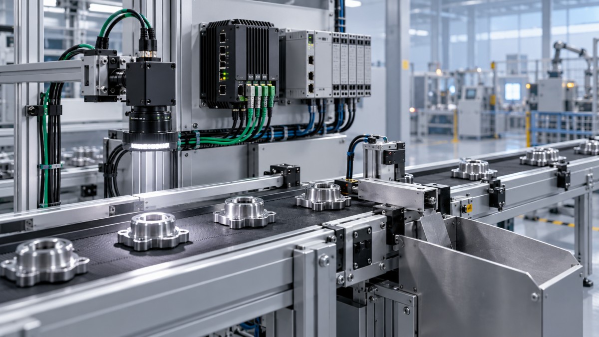
Now consider an inspection system that triggers a reject mechanism on a moving conveyor. A classification arriving after the part has passed the actuator is no longer useful. Image exposure, inference, network transport, controller scheduling, and actuator response all consume the available time. Fast Ethernet forwarding alone does not establish that the application will work.

Even within control, requirements differ. A supervisory setpoint update is not equivalent to a coordinated motion loop. Hard real-time operation requires deadlines to be satisfied under defined operating assumptions; a favorable percentile from a short benchmark is not proof of that guarantee. Safety-related functions also need their own safety assessment. Low latency does not establish functional safety.

Define exactly where the stopwatch starts and stops

A latency number without measurement boundaries is incomplete. “Gateway latency” might describe packet forwarding between interfaces, protocol conversion, or delivery from a sensor interface to an application callback. Those measurements answer different questions.

For monitoring, a useful boundary often runs from sample acquisition to availability in the consuming application. For closed-loop evaluation, extend it to the commanded physical response where that response determines success. Record intermediate timestamps where possible so delays can be attributed rather than guessed.

A practical timing path includes sensor acquisition and filtering, source-side buffering, uplink transport, gateway processing, application scheduling, decision execution, downlink delivery, and actuator response. Some stages overlap; others are strictly sequential. Build the budget around the actual implementation rather than blindly adding vendor specifications.

Sampling phase deserves particular attention. A physical change occurring just after a periodic sample may wait almost one sampling interval before acquisition begins. A benchmark starting at packet transmission excludes that wait. Likewise, a timestamp created after batch assembly can make old measurements appear newly generated.

Round-trip time is useful for diagnostics, but dividing it by two does not establish one-way latency when routes, queues, or processing differ by direction. Ask whether acknowledgments represent packet receipt, application processing, or completed action.

Clock uncertainty can overwhelm the result

One-way measurements across devices require a known relationship between their clocks. IEEE 1588 Precision Time Protocol can support precise synchronization, but its presence in a datasheet does not establish the achieved accuracy. Hardware timestamping, network asymmetry, clock configuration, and synchronization loss all affect the result.

Request the timestamp locations and measured clock-offset uncertainty during the test. If synchronization uncertainty is comparable to the reported delay, the result cannot support a fine-grained comparison. Hardware timestamps near the network interface can isolate transport behavior, while application timestamps include software delays; neither substitutes for the other.

Read the distribution, then inspect the failures

Mean latency describes central behavior, not deadline reliability. Median latency helps establish the normal operating point. Higher percentiles expose the slower portion of the distribution, while the maximum identifies the worst event observed in that particular test—not a guaranteed upper bound.

For deadline-sensitive applications, request the following alongside the histogram:

• Deadline-miss ratio: the proportion of required updates that fail to become usable before the specified deadline.
• Loss and rejection counts: including missing, duplicate, out-of-order, and expired messages.
• Consecutive misses: because a burst of failures may be more damaging than isolated late updates.
• Recovery time: how long valid, timely delivery takes to resume after a disturbance.
• Sample count and duration: needed to judge how much evidence supports the reported tail.

Define jitter explicitly. Vendors may use that term for latency standard deviation, peak-to-peak variation, or variation in packet arrival intervals. Comparing those values directly is misleading. For periodic control, arrival-time deviation relative to the expected schedule may be more actionable than a single summary statistic.

A subtle reporting problem occurs when lost messages disappear from the latency calculation. The remaining deliveries may look impressively fast even as service deteriorates. Deadline accounting should include every expected update, not only successful responses.

Also inspect latency over time. A histogram can hide bursts caused by reconnects or periodic background tasks. Zero misses in a finite run does not prove zero risk, and high-percentile estimates need enough observations to be meaningful. Correlated failures further limit conclusions drawn from simple independent-event assumptions.

Test the configuration you intend to deploy

An idle-network benchmark is useful for finding the baseline. It is weak evidence for production acceptance. Gateway timing changes when protocol translation, encryption, local analytics, logging, and store-and-forward queues compete for CPU time and memory.

Specify payload sizes, message rates, connected-device counts, directionality, and traffic patterns. Average bandwidth alone is insufficient: synchronized sensor publishing can create queue bursts even when link utilization looks modest over a longer interval. Record firmware, operating-system settings, processor power modes, and thermal conditions so the test can be repeated.

The most revealing disturbance tests usually follow the architecture. Interrupt the upstream connection if buffering is enabled. Exercise broker reconnection if messaging depends on a broker. Introduce competing traffic where links are shared. For wireless segments, evaluate representative interference and mobility conditions rather than treating a clean bench result as a coverage guarantee.

Watch what happens after connectivity returns. A gateway draining historical telemetry can delay current measurements unless traffic classes and queue policies prevent it. Reliable delivery of stale data is useful for records, but it does not restore real-time control.

Protocol and standards claims need a narrower reading

MQTT quality-of-service levels describe delivery semantics, not bounded end-to-end timing. Retransmissions and acknowledgment exchanges can change latency, while broker queues and subscriber scheduling remain part of the application path. Select delivery behavior according to whether loss, duplication, or lateness is most harmful.

OPC UA also covers different communication models. A client-server exchange and a PubSub deployment should not be treated as equivalent timing architectures. Transport selection, security configuration, implementation, and operating-system scheduling still need evaluation.

IEEE 802.1 Time-Sensitive Networking mechanisms can help engineer bounded behavior within an appropriately configured network. They do not automatically bound sensor processing, gateway software, or actuator response. Ask which mechanisms are implemented, how traffic is admitted and scheduled, and which network assumptions underpin any timing claim.

The distinction matters in supplier comparisons: protocol support establishes capability, while a documented configuration and test establish evidence for a particular use.

Turn the measurements into an acceptance specification

Start with the process deadline and work backward. As an illustrative budget—not a recommended universal limit—suppose a sensing-to-action deadline is 10 milliseconds. If acquisition, computation, and actuation together consume 6 milliseconds under the defined conditions, transport and remaining scheduling must fit within the balance, with uncertainty and engineering margin accounted for. A 3-millisecond average network delay would not, by itself, demonstrate compliance.

An acceptance specification should identify the start and end events, timestamp method, allowable measurement uncertainty, operating envelope, and required deadline behavior. It should also define test duration, disturbance scenarios, loss accounting, and the response to stale data. Separate normal-operation acceptance from degraded-mode requirements instead of blending both into one percentile.

Specify what the application does when the deadline cannot be met: discard an expired command, hold a previous value where permitted, enter a defined fallback mode, or transfer responsibility to a local controller. The right behavior depends on process dynamics and hazard analysis. It should not be left to a messaging library’s default queue policy.

This is where TechStat Vanguard’s data-driven benchmarking approach is most useful: separating measured capability from assumptions and unsupported claims. A defensible comparison retains raw timing traces, configuration details, and test limitations—not merely a ranking by average latency.

If a supplier cannot explain timestamp boundaries, losses, and behavior under load, treat its latency figure as preliminary. Keep tightly constrained control local unless the complete proposed path has adequate evidence. Use broader connectivity for the monitoring and supervisory functions it can demonstrably support, then test the remaining timing risks before committing the architecture.